Wavelets II - Vanishing Moments and Spectral Factorization

• Audio DSP
• wavelet
• Tutorials

In the previous blog post I described the workings of the Fast Wavelet Transform (FWT) and how wavelets and filters are related. As promised, in this article we will see how to construct useful filters. Concretely, we will find a way to calculate the Daubechies filters, named after Ingrid Daubechies, who invented them and also laid much of the mathematical foundations for wavelet analysis.

Besides the content of the last post, you should be familiar with basic complex algebra, the Fourier transform, Taylor series and binomial coefficients. Just to get started, we recall that the scaling function $\phi$ and the wavelet function $\psi$ are defined by the filter coefficients $h_0$ and $h_1$ via the dilation/refinement equations:

Vanishing Moments and Continuous Functions

The idea of vanishing moments is the additional ingredient we need to create our wavelet functions. In our implementation of the FWT, the input signal $x(t)$ is split in two parts. As limit for the late stages, one part was analyzed with $\psi$ and one was analyzed with $\phi$. If $\psi$ is orthogonal to $x(t)$, i.e. $\int x(t) \psi(t) \mathrm{d}t = 0$, then the whole signal is represented by the $\phi$ half and can nevertheless be perfectly reconstructed. This scenario is of course great for compression, and in general for data manipulation or analysis. So one measure of quality of the wavelet function $\psi$ is, to how many important functions it stands orthogonal to. In the case of so-called vanishing moments these important target function are polynomials.

The $n$th moment of a function $f$ is defined as:

If this moment vanishes, then $f(t)$ is orthogonal to $t^n$. If we say a function has $A$ vanishing moments, we usually mean it has vanishing moments $M_n = 0$ for $n=0, 1, ..., A-1$. Because of the linearity of the integration operation, this means that the function is orthogonal to all polynomials up to degree $A-1$:

If the wavelet function $\psi$ has a certain number of vanishing moments, then discretely shifted versions of $\phi$ can be used to reconstruct all the polynomials that $\psi$ stands orthogonal to. For $A=1$ this is clear: we can analyze a constant signal with the Haar scaling function, which is simply a rectangle. The synthesis scaling function looks exactly the same and the signal can be reconstructed.

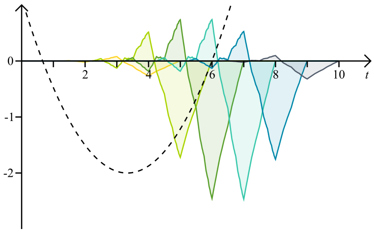
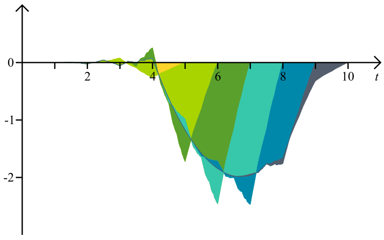
With $A=2$, things are not as obvious. A linear signal cannot be constructed by simply adding together fixed line segments since it has to work for all slopes. But the Daubechies 4 (DB4) functions that we saw in the last post have exactly this property, i.e. two vanishing moments.

It seems a bit strange that these odd spiky scaling functions sum up to a smooth straight line. But if we add one at a time, we see that they fit together like the pieces of a puzzle to reconstruct a (shifted) segment of the original signal. The DB6 wavelet has three vanishing moments ($A=3$). So any quadratic signal can be constructed with the DB6 scaling function:

Polynomials of high degrees can approximate many different signals. This means a wavelet function $\psi$ with many vanishing moments stands orthogonal or almost orthogonal to a wide range of different signals. The corresponding scaling function $\phi$ in turn has the expressive power to reconstruct all these signals. This is of course a highly desirable property, and there exist wavelets with any number of vanishing moments. In the rest of this post we will see how to construct the filters resulting in these wavelets. The downside is, as it turns out, that for more vanishing moments we need longer filters in the FWT implementation.

Vanishing Moments and Discrete Filters

In a FWT we do not explicitly use the functions $\phi$ and $\psi$, instead they emerge from the filters $h_0$ and $h_1$. We have to transfer the idea of vanishing moments to these filters. To do this, we plug the wavelet equation $(2.2)$ into the moment definition $(2.3)$ and let the moments vanish:

We assume that $\phi$ has the necessary moments, but they are not zero. Now we create a new variable $s_k := 2t-k$:

Let’s look at $(2.4)$ for the first few moments:

$n = 0$:

The integral $\int \phi(s_k) \mathrm{d}s_k = \int \phi(2t-k) \mathrm {d}t$ is invariant to changes in $k$, so $M_n(\phi(s_k))$ is constant for all $k$. With that, the requirement for one vanishing moment is:

$n = 1$:

The second term $\sum_k h_1(k) \frac{1}{2} M_1(\phi(s_k))$ is zero, we know that from the condition for the $0$th vanishing moment. From the second term $\sum_k h_1(k) \frac{1}{2} k M_0(\phi(s_k)) = 0$ follows the new condition for vanishing moment $1$:

$n = 2$:

Now both the second and third term are zero, based on the previous conditions. And the new condition for vanishing moment $2$ is:

In general, for every new vanishing moment $n$, there will be a term proportional to $\sum_k h_1(k) k^n M_n(\phi(s_k))$. All other terms will have a factor $k^m$ with $m<n$, those will automatically zero, based on the previous conditions. With that we have the condition for filter coefficients $h$ of a wavelet function $\psi$ with $A$ vanishing moments:

Or, because $h_1 = -(-1)^k h_0(L-1-k)$, see $(1.6)$:

We see from $(2.3)$ that the concept of vanishing moments is directly applicable to discrete filters, $h_1$ stands orthogonal to all polynomials up to degree $A-1$. This means, in a Fast Wavelet Transform (FWT) setup those functions are arbitrarily compressible!

Filter Construction in the Frequency Domain

Recall that we only need to construct $h_0$ for our FWT, the other three filters $h_1$, $f_0$ and $f_1$ then emerge from the rules $(1.4)$ - $(1.6)$. For $h_0$ we now have two constraints:

• $\sum_n h_0(n)h_0(n + 2k) = 2 \delta (k) = \begin{cases} 2, \; k = 0 \\ 0, \; k\neq 0 \end{cases}$, this is the shift orthogonality condition $(1.8)$ that guarantees perfect reconstruction.

• $\sum_k k^n (-1)^k h_0(k) = 0; \: \: n = 0, 1, ..., A-1$, which we just saw, where we can set $A$ to be the number of vanishing moments we want.

These two conditions yield the famous Daubechies wavelets. Unfortunately, the construction is quite fiddly, we will need some complex algebra and Fourier analysis, a bit of number theory and a little combinatorics. But I hope this is interesting and in the end we will arrive at a relatively simple algorithm. If you want, you can now first take a look at this algorithm and then read on from here to find out why it works.

We now have to move to the frequency domain, and because some trigonometric identities will turn out to be helpful we use the Fourier transform instead of the z-transform. By definition, the Fourier transform of $h_0$ is

We already know the z-transform of the shift orthogonality condition. This was equation $(1.7)$ from the last article. Converting between the z- and Fourier transform is done using $z = e^{i \omega}$ and therefore $-z= \overline{e^{i(\omega+\pi)}}$ as well as $z^{-1}=e^{i \omega}$. Because $h_0(k)$ are real values, there also is $H_0(-z) = \overline{\hat{H_0}(\omega + \pi)}$ and $H_0(z^{-1}) = \overline{\hat{H_0}(\omega)}$. This means we can write

Now we need to convert the vanishing moment condition to the frequency domain. We can write the $n$th derivative of $(2.7)$ as

If we set $\omega = \pi$, we get $(D^n \hat{H_0})(\pi) = (-i)^n \sum_k k^n (-1)^k h_0(k)$. This means

is equivalent to $(2.6)$ and $(2.5)$.

The easiest way to achieve $(2.9)$ would be setting $\hat{H_0}$ to $(1 + e^{-i \omega})^A$. This unfortunately interferes with $(2.8)$. But if we multiply $(1 + e^{-i \omega})^A$ with an arbitrary function $L$, then $(2.9)$ still holds because of the product rule. We want our coefficients $h_0$ to be real values, this means $L$ would have to be a polynomial with real coefficients in $e^{i\omega}$ as well. This means we can set

and only need to search for a function $L(e^{i\omega})$ so that $(2.8)$ is satisfied (we have divided the base of the first factor by 2, you will see why straightaway).

Now we need our trigonometric identities. $(2.10)$ in combination with $\left| \frac{1+e^{-i\omega}}{2} \right|^2 = \frac{1 + \cos(\omega)}{2} = \cos^2 \left( \frac{\omega}{2} \right)$ gives us

We can see directly from $(2.7)$ that $\hat{H_0}(-\omega) = \overline{\hat{H_0}(\omega)}$. This makes $\left| \hat{H_0}(\omega) \right| ^2$ an even function, which means it is symmetric with respect to $\omega = 0$ and can be expressed in terms of only cosine-functions. The same has then to be true for $\left| L(e^{i\omega}) \right| ^2$. With $\cos(\omega) = 1 - 2\sin^2(\frac{\omega}{2})$ and $P$ being a polynomial we can write:

Now we can write the shift orthogonality condition $(2.8)$ as

If we set $y = \sin^2(\frac{\omega}{2})$, which also means $1-y = \cos^2(\frac{\omega}{2})$, we can write this as

Bezout’s Identity

We are now probably at the most abstract point of the wavelet construction. Why all this effort to get a equation in the form of $(2.12)$? The reason is number theoretical result called Bézout’s identity. You can read about it further elsewhere, but in our case it says that there exists a polynomial $P(y)$ of degree $A-1$ so that $(2.12)$ is true. How exactly it looks like, however, we have to find out ourselves. First we solve for $P(y)$:

The second term has a factor $y^A$, so there is no way we can model it with a polynomial of degree $A-1$. The best we can do is create a Taylor expansion at $y=0$ of the first term $4(1-y)^{-A}$. For a function $f(y)$, a Taylor approximation at $y=0$ means

Our $f(y)$ is $4(1-y)^{-A}$ as we said. We can write out its $n$th derivative:

This means the coefficient of $y^n$ in our Taylor series is

Now we can write out our solution for $P$:

Verifying that this indeed is a solution of $(2.12)$ is not trivial, but it can be done. We define

We now need to proof that $S_{A-1}$ is $1$ for all $A$.

Here we have multiplied every term with $((1-y)+y) = 1$, which of course is a legitimate thing to do. If we expand these products, we can write

Let’s just look at $\sum_{k=0}^{n} {A-1+k \choose k}$:

From this we see that

Now we have

Because $2 {2A-1 \choose A-1} = \frac{2A \: (2A-1)!}{A\: (A-1)!(A)!} = {2A \choose A}$ this means

and by induction $S_{A}(y) = S_{A-1}(y) = ... = S_{0}(y) = 1$.

Spectral Factorization

Now it is time go back and basically reverse all steps to get our coefficients $h_0$. With the result $(2.14)$ and $(2.11)$ we have

We have defined $y = \sin^2(\frac{\omega}{2}) = (1-\cos(\omega))/2 = \frac{1}{2} - \frac{1}{4}(e^{-i\omega} + e^{i\omega}) = \frac{1}{2} -\frac{1}{4}(z + z^{-1})$, this means

From this we need to find $L(z)$. Like any polynomial, $L$ can be factorized as

where $z_k$ are the roots of $L(z)$ and $c$ is a scaling constant. This obviously means

From $(2.8)$ in combination with $(2.5)$ we see that $\left| H(1) \right| ^2 = 4$, which means $H(1) = 2$ and $L(1) = 2$. To get this, we wet set $c := 2 \left( \prod_{k}(1-z_k)\right)^{-1}$. If we compare $(2.17)$ and $(2.18)$, we see that they fit together: The roots in $(2.17)$ come in reciprocal pairs, which is just what we want for $(2.18)$. To get $L(z)$, we need one half of the roots of $(2.17)$. If we don’t want to find the roots of a rational function, we can define the polynomial

which means $\left| L(z) \right| ^2 = 4 Q(z)z^{-(A-1)}$ and find the roots of $Q$. We can do this because the factor $4 z^{-(A-1)}$ leaves the existing roots untouched and does not introduce any new roots, since itself has none.

As we said, for any root of $Q$, its reciprocal will automatically be a root too. To get the correct $L$, we have to select only one of each pair as $z_k$. If a root is complex, we also have select its complex conjugate, which will also be a root, to get real coefficients. A simple way to meet both of these conditions is to only select the roots inside the unit circle, meaning its absolute value is less than or equal to 1. This will give us the original Daubechies coefficients. Because $Q$ has $2(A-1)$ roots, $L$ will have a degree of $A-1$. With the roots $z_k; \; k=1, ..., A-1$ selected, we have

and with $(2.10)$

Expanding this into the form

gives us the filter coefficients we are looking for. As we see, a Daubechies filter with $A$ vanishing moments has $2A$ coefficients.

Algorithm for calculating Daubechies coefficients

• Define $A$ as the number of vanishing moments you want from your filters
• Calculate the roots of the polynomial $\sum_{n=0}^{A-1} {A + n - 1 \choose \:n} \: \left( \frac{1}{2} -\frac{1}{4}z - \frac{1}{4} z^{-1} \right)^n z^{A-1}$. Do this with your favourite math library, or implement an algorithm that finds the roots using Newton’s method.
• Set $z_k$, where $k=1, ..., A-1$, to the roots inside the unit circle, i.e. $\left| z_k\right| \leq 1$ must be true for all $k$.
• Expand the polynomial $H_0(z) = 2 \left( \frac{1+z}{2}\right)^A \prod_{k=1}^{A-1}(z-z_k)(1-z_k)^{-1}$ into the form $H_0 = \sum_{n=0}^{2A-1} h_0(n)z^n$. The values $h_0$ are the coefficients of the lowpass analysis filter.

Example: Calculating the DB6 coefficients

We set $A=3$, this give us the polynomial

As we see, the real part is symmetric and the imaginary part is antisymmetric with respect to the real axis. Two roots (the small white spheres) lie inside, two outside the unit circle.

We can ask WolframAlpha for the roots and get the solutions $0.28725 - 0.15289 \:i$, $0.28725 + 0.15289 \:i$, $2.7127 - 1.4439 \:i$ and $2.7127 + 1.4439 \:i$. Actually, in this case there exist exact solutions, but they are a bit unpractical for this demonstration.

We set $z_1 = 0.28725 - 0.15289 \:i$ and $z_2 = 0.28725 + 0.15289 \:i$ because they are complex conjugates and have an absolute value smaller than 1. Now we have

That gives us the DB6 coefficients:

Conclusion

We saw the significance of vanishing moments to continuous wavelets as well as to the filters of a FWT implementation (these filters define wavelets with the same number of vanishing moments via $(2.2)$). They make sections of signals that resemble polynomials highly compressible and very easy to handle. We then derived an algorithm to calculate Daubechies filter with any number of vanishing moments. This was done by bringing the shift orthogonality and the vanishing moment condition to the frequency domain, resulting in equations $(2.8)$ and $(2.9)$. We combined them to $(2.12)$, which we were able to solve using Bezout’s identity. To get back to $H_0(z)$, we used a procedure called spectral factorization. We factorized $H_0$ using the roots of the polynomial we found earlier.

In practice, you probably won’t need to calculate the Daubechies coefficients, they are available online from DB2 to at least DB20. But there are many other wavelets with pros and cons for different applications. With these two articles you should have the background to understand most papers explaining them, or even invent new wavelets yourself.

For the next post, I am planning to write about the Dual Tree Wavelet Transform, which uses complex wavelets. It is currently mainly used in image recognition, but I think it also has great potential for audio processing. But I am open to suggestions for the next topic as well! Again, any feedback is appreciated. Thank you for reading!

Useful Resources

• Daubechies, Ingrid: Orthonormal bases of compactly supported wavelets (link to pdf)
• Daubechies, Ingrid: Ten Lectures on Wavelets
• Keinert, Fritz: Wavelets and Multiwavelets
• Mallat, Stéphane: A Wavelet Tour of Signal Processing
• Rieder, Andreas: Wavelets - Theory and Applications
• filter coefficients of many different wavelets (all coefficients are scaled by a factor of $2^{-1/2}$)

Sign in