Wavelets I - From Filter Banks to the Dilation Equation

• Audio DSP
• wavelet
• Tutorials

This is the first in what I hope will be a series of posts about wavelets, particularly about the Fast Wavelet Transform (FWT). The FWT is extremely useful in practice and also very interesting from a theoretical point of view. Of course there are already plenty of resources, but I found them tending to be either simple implementation guides that do not touch on the many interesting and sometimes crucial connections. Or they are highly mathematical and definition-heavy, for a non-mathematician (such as me) it might be difficult to distill the important ideas. I will try to cover all necessary aspects as clearly as possible, so that we get to a point where we can work confidently and creatively with these algorithms.

Here we will start with the implementation of the FWT, which is easily done with a cascaded filter bank. From there we develop the corresponding wavelet properties and get to the maybe most important aspect of the Multi-Resolution Analysis (MRA), namely the dilation and wavelet equations. I think this is a reasonable and intuitive approach, although I have not seen it like that anywhere else. My assumption is that you know the very basic principles of the continuous wavelet transform, digital filters and the Z-transform. I just want to mention that this is my first post of this kind in English and I would appreciate your comments if you find mistakes in this text or in the calculation, if something is unclear or if you have any kind of feedback or question!

Filter Banks

A finite impulse response (FIR) filter transforms a discrete signal $x(n)$ by convolving it with a finite series of values $h(k)$:

The basic building block of our filter bank is shown in this graphic:

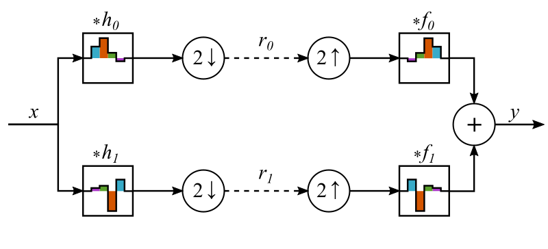
The input signal $x(n)$ is split and fed into two different analysis filters $h_0$ and $h_1$. These two signals are downsampled by a factor of two (i.e. all values with odd $n$ are deleted). Now we have an intermediate representation of the input signal, consisting of two different signals $r_0$ and $r_1$, each with half the sample count. But if we do it right, since the total amount of samples remains the same, there could still be all information left from the input. To reconstruct the signal, the representations are now upsampled by a factor if two (a zero is inserted after each sample) and fed into the reconstruction filters $f_0$ and $f_1$. Then the outputs of these filters are added together.

If possible, we want the output of this whole setup to be exactly the same as the input, except maybe a constant gain and delay, making it a perfect reconstruction (PR) filter bank. The simplest set of filters meeting this condition are the Haar filter: $h_0 = [1, 1]$, $h_1 = [-1, 1]$, $f_0 = [1, 1]$, $f_1 = [1, -1]$. You can check it yourself by feeding a single impulse signal ($x = [..., 0, 0, 1, 0, 0, ...]$) into the filter bank and seeing that the output is still an impulse. Because of the linearity of the system this means that signals, since they are just a linear combination of many impulses, will be perfectly reconstructed.

Of course there are not just the Haar filters that yield a PR filter bank. Let’s look at the Z-transform of Figure 1:

More information is available here. Our PR condition, with gain $g$ and a delay of $d$ samples, in terms of the Z-transform is

As we see, there is no use for the second term in $(1.2)$, i.e. the alias term proportional to $X(-z)$. The easiest way to get rid of it is to set

• $F_0(z) = -H_1(-z)$, which is equivalent to $f_0(n) = -(-1)^n h_1(n)$ $(1.4)$

• $F_1(z) = H_0(-z)$, which is equivalent to $f_1(n) = (-1)^n h_0(n)$ $(1.5)$

To have everything nice and compact we set $h_0$ and $h_1$ to be a so-called conjugate quadrature filter (CQF) pair. Here this means $h_1$ is $f_1$ in reverse ($L$ is the length of $h_0$ and must be even):

• $H_1(z) = z^{-(L-1)} F_1(z^{-1}) = -z^{-(L-1)} H_0(-z^{-1})$, or $h_1(n) = -(-1)^n h_0(L-1-n)$ $(1.6)$

Now $f_0$, $f_1$ and $h_1$ can be all expressed in terms of $h_0$. An additional benefit is that $h_0$ and $h_1$ are orthogonal:

Equation $(1.2)$ combined with the PR condition $(1.3)$ becomes:

If we set $d=L-1$ and $g=-2$, we can write

This constraint is not quite as straightforward to translate for $h_0$. Using the definition of the Z-transform we can write

Because it can’t depend on $z$, $\sum_n h_0(n)h_0(n+m)$ has to be zero for $m \neq 0$. With $k := \frac{1}{2}m$, our perfect reconstruction constraint for $h_0$ is:

Which means $h_0$ has to be orthogonal to versions of itself shifted by an even number of samples. This orthogonality condition, in combination with $(1.4)$, $(1.5)$ and $(1.6)$ is sufficient for creating a set of filters for a PR filter bank. A procedure for getting the $h_0$ coefficients with additional beneficial features will be explained in my next blog post.

As you can see, I use specific filters in the graphics. These are the filter coefficients of the Daubechies 4 (DB4) wavelet, each one in a different color.

$h_0(0) = 0.6830127$
$h_0(1) = 1.1830127$
$h_0(2) = 0.3169873$
$h_0(3) = -0.1830127$

You can check that they meet the $(1.8)$ condition. I picked these because of the manageable filter length of four, and their characteristic shape. My aim is to anchor the abstractions with some concrete elements and thus making it easier and more intuitive to grasp.

The representations $r_0$ and $r_1$ are themselves signals that can be fed into a similar filter bank module. We can do this an arbitrary number of times, resulting in more and more representations of coarser and coarser resolution.

Reconstruction works the same way. And if all filter bank modules reconstruct the signal perfectly, so does the whole cascade.

Multi Resolution Convolution

In this section we will concentrate on the $h_0$ filter. So let’s look at the upper half of Figure 2 (shaded in yellow). What has to happen to compute one sample, say the one with index 0, of the representation signal $r_{000}$? We can draw a graph describing the operation as a computational graph:

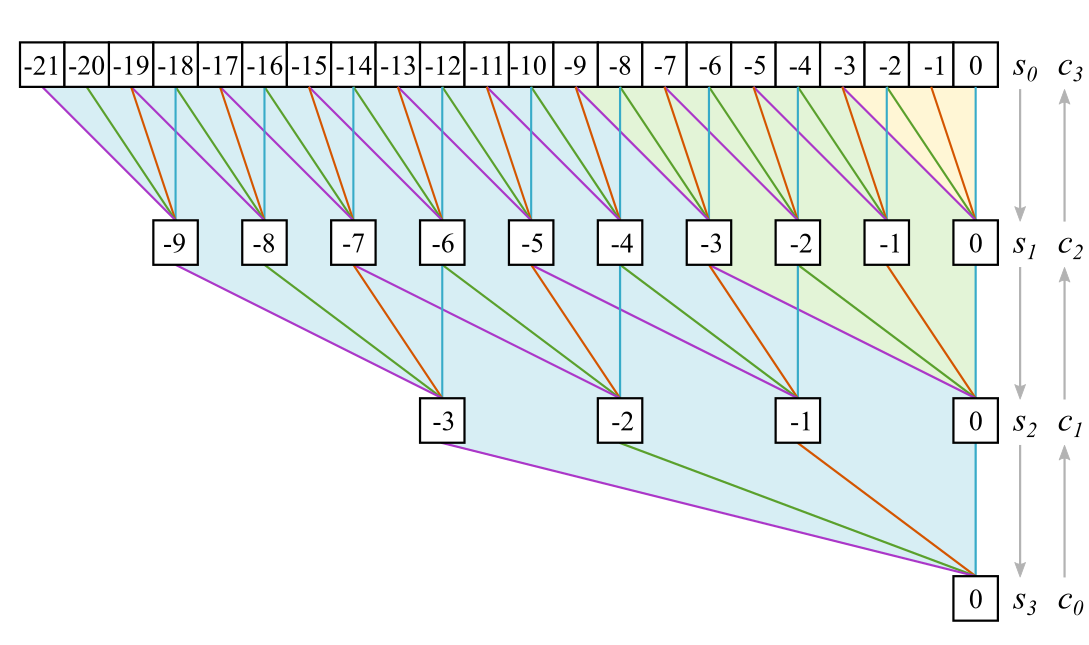
The white squares illustrate the signal at different representation states, which I have slightly renamed for convenience: $s_0 = x, s_1 = r_0, s_2 = r_{00}$ and in general $s_i$ being the representation $r$ with $i$ subscript zeros, meaning the output of the $i$th analysis filter $h_0$. A colored line stands for a multiplication with the corresponding filter coefficient, following the specified convolution and downsampling procedure

It should be clear how the graph would look like if we added more layers and looked at the sample 0 of the innermost representation signal. The graph would grow upwards, getting denser and denser at the top, but the bottom part stayed the same, only the labels of the representations would change.

Technically, our topic is wavelets. At their core idea, wavelet representations do not build on one another. A scaled and shifted version of a wavelet is used always on the original signal, the cascading approach is just an implementation trick. This means for our filter bank it is also useful to examine how the direct link from the signal to every representation level looks like. For that, we have to look at Figure 4 in a different way: All the operations for generating the bottom sample 0 from the input signal $x$ - since they are all linear - can be combined into a single long filter $c_n$, where $n$ is the number of considered representation stages. To get the coefficients of this combined filter, we look at all the paths connecting a square at the level $c_n$ to the bottom square. These paths all have $n$ colored segments. The coefficients corresponding to the color of the segments are multiplied and these products are added for each different path. Note that now the white squares don’t depict the signal in its various representations anymore, but the coefficients of the combined filter $c_n$. For example, if we take $c_3[-10]$, there are four paths to $c_0[0]$:

This results in a filter coefficient

The resulting factor is exactly how an input sample is scaled while traveling through the graph from top to bottom.

The efficient way to compute the coefficients for $c_n$ is working the way up the graph and using the following rule (all values of $c_n$ with non-integer indices are zero):

The length of the filter $c_n$ more than doubles for each subsequent level. To again get closer to the idea of wavelets, which are first defined at a certain size and then scaled, we do not want an ever growing discrete filter, but rather a function that ideally will be continuous at the limit. To achieve this, we have to introduce a re-parametrization of the filter: $x_n(t_n) = c_n(j)$, where $t_n = -2^{-n}j$, which also means $t_n = 2t_{n+1}$.

We have to adapt our construction progression for the filter functions $x_n$:

Or when we set $t := t_{n+1}$

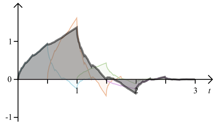
We have to give this sequence a starting value, we use $x_0(0) = 1$. Then $x_1$ has just the $h_0$ filter coefficients as values. The next graphic shows the first several levels of $x$ and the converged progression:

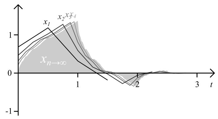
These are, in the sense of a discrete continuous wavelet transform, the actual “wavelets” used, for each representation a different one, although they converge quite quickly.

The Dilation Identity

The $2^{-n-1}$ factor in $(1.11)$ prevents this progression from being elegantly expressed as a limit for $n \to \infty$. So we will try to find a better suited equivalent progression. The first step, calculating $x_1$ from $x_0$, could also be achieved by $x_1(t) = \sum_k h_0(k) x_0(2t - k)$, as we can easily see. This currently seems somewhat arbitrary, but let’s generalize this relation nevertheless to a construction progression of different function $\phi$:

Notice that it has the same form as $(1.9)$. I think this resemblance can be a bit misleading, as blurs the distinction between the filter bank implementation and the underlying mathematical framework of the MRA. Looking at the corresponding graph shows that the link between $x_n$ and $\phi_n$ is less obvious at it may seem at the first superficial glance:

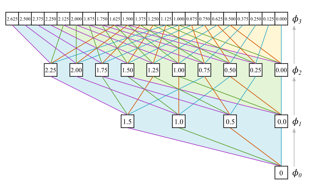
The connections are completely different from the previous graph, except for the first step. But the remarkable thing is that the paths connecting values of $\phi_n$ to $\phi_0$ have exactly the same color combinations as the $x_n$ graph. See for yourself! We can look again at $\phi_3(1.250)$, which is equivalent to our previous example $c_3(-10)$. The paths connecting this node to $\phi_0(0)$ are:

And with that we have

The order of the paths is jumbled, as are the colors of the path segments (those are in fact exactly reversed). But in the end they generate the same result. But while we can verify the identity $\phi_n(t) = x_n(t)$ for $n={1, 2, 3}$, this seems a bit magical and is nothing more than a nice observation. We need a proof that the identity holds for all $n$.

Let’s start with our two progressions $(1.11)$ and $(1.12)$:

We assume that $x_n = \phi_n$. They are now interchangeable and we swap them.

Then we go back one more level and plug in the recursive step that defines $\phi_n$ or $x_n$ in terms of $\phi_{n-1}$ or $x_{n-1}$.

As we see, the arguments of $\phi_{n-1}$ and $x_{n-1}$ on the right are the same. This means, if we additionally assume $\phi_{n-1} = x_{n-1}$, then $\phi_{n+1} = x_{n+1}$. In short:

If $\phi_{n} = x_{n}$ and $\phi_{n-1} = x_{n-1}$, then $\phi_{n+1} = x_{n+1}$

We have already seen that our assumptions hold for the first two levels, i.e. $\phi_0(t) = x_0(t)$ and $\phi_1(t) = x_1(t)$. With that, as we showed, we have $\phi_2(t) = x_2(t)$, and as a consequence of that $\phi_3(t) = x_3(t)$, and so on for all $n$. Therefore we have proved by induction that indeed:

$\phi_n(t) = x_n(t); \; n \geqslant 0, t \in R$, if $\phi_0(0) = x_0(0) = 1$ and $\phi_0(t) = x_0(t) = 0; \forall t \neq 0$ $(1.13)\;\;\;$

The Dilation and Wavelet Equation

For $n \to \infty$, $\phi_n$ converges to a continuous function with support $[0, K-1]$, where $K$ is the number of coefficients of $h_0$, and $x_n(0) = x_n(K-1) = 0$ (the support of a function is the interval where it is different from zero). Let’s call this function simply $\phi$. This converged progression still has to hold the construction criterion:

This is the dilation equation, the workhorse in the theory of the FWT and MRA. And $\phi$ itself is the scaling function of the FWT, in our concrete examples the DB4 scaling function. The dilation equation says that the scaling function has a fractal self-similarity: it can be constructed of versions of itself, compressed by a factor of two, shifted and scaled by the $h_0$ coefficients.

We of course have a way to approximate $\phi$ by iterating (1.12). This is called the cascading algorithm, and the iterations will, as we showed, look exactly like in Figure 6. While it is not possible to write the scaling function out explicitly, we can get can exact values by solving a system of linear equations derived from the dilation equation.

or

This system is homogeneous, meaning it has only zeros on the right side, and has no distinct solution. We have modify it slightly:

I have added the first and last equation together and added an additional constraint, namely that the sum of the four variables should be 1. This system can be solved and gives us the values of $\phi$ at the four integer positions. We plug these values in the dilation equation to get the values that lie exactly halfway between them and repeat this procedure. This way we have very quickly a large amount of exact values of $\phi$.

We have not yet looked at the signal representations obtained with the $h_1$ filter, the $r_{...1}$ in Figure 2. We cannot define something like a scaling function for $h_1$, because the cascading algorithm does not converge for a highpass filter. But we can easily see what happens if we analyze a representation that itself was constructed with the $h_0$ scaling function $\phi$ (so basically one pass through the $h_1$ filter after infinitely many passes through $h_0$). For this we take the proof leading to $(1.13)$ and use it with adapted progressions:

The proof works just the same, and we can write:

This is the wavelet equation, defining the wavelet function $\psi$ of our FWT. According to the this equation, the wavelet function $\psi$ can also be constructed from compressed and scaled version version of $\phi$, this time scaled by $h_1$.

The thing last to show in this article is that not only $h_0$ and $h_1$ are orthogonal, which as we saw arises from $(1.6)$, but also $\phi$ and $\psi$:

First we used the linearity and shift invariance of the integration operator to group the function into multiple terms. Then we can see that the factors of all terms are zero, because of the relationship between $h_0$ and $h_1$ defined in $(1.6)$.

Conclusion

We have seen the conditions $(1.4)$ - $(1.8)$ for the analysis filters $h_0$ and $h_1$, as well as the synthesis filters $f_0$ and $f_1$ of a cascaded perfect reconstruction filter bank implementation of the FWT. Those are critical and sufficient to make it work. Then we have tried to look at this implementation from a wavelet point of view. For this we have introduced the identity $(1.13)$, which then led to the dilation equation $(1.14)$ and wavelet equation $(1.15)$. Those equations define the functions $\phi$ and $\psi$ in terms of the filters $h_0$ and $h_1$.

The scaling function $\phi$ and the wavelet function $\psi$ give us a great analytic perspective of our algorithm. But it is important to remember that they are theoretical limits that never actually occur in a practical filter bank implementation of the FWT, not even as discretized or subsampled versions. This is a distinction from a discrete implementation of the continuous wavelet transform, where the scaled wavelets are explicitly used.

The fact that the actually (implicitly) used filters $\phi_n$ with finite $n$ vary from $\phi$ can be seen as a discretization artifact. A signal with higher sample rate uses a better approximation of $\phi$ at a certain scale, because it must have gone through more precedent filters to reach this level. If we could use the filter banks on a infinitesimally sampled signal, all filters would have had an infinite count of filters before them, making the effective filter be equal to $\phi$.

This concludes my first article. I hope it was interesting for now, although it might not yet be clear how we can actually use these results. In the next blog post, however, I will explain how they can help us to design better filters with remarkable features.

Useful Resources

• Blatter, Christian: Wavelets - Eine Einführung (link to pdf, german)
• Fugal, D. Lee: Conceptual Wavelets
• Keinert, Fritz: Wavelets and Multiwavelets
• Rieder, Andreas: Wavelets - Theory and Applications
• Smith III, Julius O.: Spectral Audio Processing
• Strang, Gilbert: Wavelets and Dilation Equations: A Brief Introduction (link to pdf)
• Winkler, Joab A.: Orthogonal Wavelets via Filter Banks: Theory and Applications (link to pdf)

Sign in