Frequency Translation by Way of Lowpass FIR Filtering

• Tips and Tricks

Some weeks ago a question appeared on the dsp.related Forum regarding the notion of translating a signal down in frequency and lowpass filtering in a single operation [1]. It is possible to implement such a process by embedding a discrete cosine sequence's values within the coefficients of a traditional lowpass FIR filter. I first learned about this process from Reference [2]. Here's the story.

Traditional Frequency Translation Prior To Filtering

Think about the process shown in Figure 1. First, an $ x(n) $ input sequence is multiplied by a $ cos (2 \pi n f_t/f_s) $ sequence which translates $ x(n)'s $ spectral components both up and down in frequency by $ f_t $ Hz. (The 't' subscript in $ f_t $ means "translation" and $ f_s $ is the input data sample rate in Hz.) Following that, the frequency-translated sequence is lowpass filtered by a six-coefficient lowpass FIR filter. Note that the high-frequency spectral components generated by the cosine mixing are attenuated by the lowpass filter.

Figure 1: Traditional frequency translation followed
by a fifth-order lowpass filtering.

The Figure 1 'frequency translation and filtering' operation can be implemented as shown in Figure 2, where no cosine multiplier is needed. The Figure 2 filter, what I call a " Translating FIR Filter ", has integer N unique set of coefficients. (I show how to select the value N in a later section of this blog.)

Figure 2: Fifth-order lowpass Translating FIR
Filter requiring N Coefficient Sets.

As each new $ x(n) $ input sample arrives to the filter the rotary switches jump to the next "Coefficient Set". (After the last $ h_N(k) $ Coefficient Set is used, when the next $ x(n) $ sample arrives we switch back to first Set $ h_1(k) $ Coefficient.) Justification for why the Figure 2 filter is equivalent to the Figure 1 filter is given in Appendix A.

Computing the Coefficient Sets' Coefficient Values

Assuming the Figure 1 FIR filter has integer K coefficients, the Figure 2 Translating FIR Filter's coefficients are the Figure 1 $ h(k) $ coefficients multiplied by time-shifted versions of the $ cos(2 \pi n f_t / f_s) $ sequence. That is, the first $ h_1(k) $ Coefficient Set's K coefficients are defined by:

\begin{eqnarray} h_1(n) & = & h(0)cos(2 \pi (0) f_t / f_s), \ h(1)cos[2 \pi (-1) f_t/f_s], \ h(2)cos[2 \pi (-2) f_t/f_s], \\ & & h(3)cos[2 \pi (-3)  f_t / f_s], ..., h(K-1)cos\{2 \pi [-(K-1)]f_t / f_s\}. \end{eqnarray}

The second and third Coefficient Sets' K coefficients are defined by:

\begin{eqnarray} h_2(n) & = & h(0)cos(2 \pi (1) f_t / f_s), \ h(1)cos[2 \pi (0) f_t/f_s], \ h(2)cos[2 \pi (-1) f_t/f_s], \\ & & h(3)cos[2 \pi (-2)  f_t / f_s], ..., h(K-1)cos\{2 \pi [-(K-1)+1]f_t / f_s\}. \end{eqnarray}

\begin{eqnarray} h_3(n) & = & h(0)cos(2 \pi (2) f_t / f_s), \ h(1)cos[2 \pi (1) f_t/f_s], \ h(2)cos[2 \pi (0) f_t/f_s], \\ & & h(3)cos[2 \pi (-1)  f_t / f_s], ..., h(K-1)cos\{2 \pi [-(K-1)+2]f_t / f_s\}. \end{eqnarray}

The Nth Coefficient Set's K coefficients are defined by:

\begin{eqnarray} h_N(n) = & h(0) & cos(2 \pi (N-1) f_t / f_s), \ h(1)cos[2 \pi (N-2) f_t/f_s], \\ & h(2) & cos[2 \pi (N-3) f_t/f_s], \ h(3)cos[2 \pi (N-4)  f_t / f_s], \ ..., \\ & h(K & -1) cos\{2 \pi [-(K-1)+N-1]f_t / f_s\}. \tag{1} \end{eqnarray}

Don't let the above equations trouble you--they are straightforward. For example, for a 6-tap (K=6) FIR filter requiring N=8 Coefficient Sets, the six cosine indexing factors inside the parenthesis in the above equations are shown in the rows of the following table.

Cosine index factors in Eq. (1) for K=6 and N=8

How Many Coefficient Sets Are Needed?

The number of necessary Coefficient Sets, N, is unrelated to the number of coefficients in the original Figure 1 FIR filter. The number of necessary Coefficient Sets for the Figure 2 implementation is given by:

where I is an integer that forces N to be an integer. For example, if your desired translation frequency is f_t =2f_s/9 Hz, making the ratio f_s/f_t =9/2, then the integer I is chosen to be I= 2 so that:

$$ N = \frac{f_sI}{f_t}=\frac{9(2)}{2} =9  \text{ Coefficient Sets.}$$

If you decide to implement a Translating FIR Filter, Appendix B lists several issues you should keep in mind.

Decimating With Translating FIR Filters

Implementing decimation (downsampling) with a Translating FIR Filter is the process shown in Figure 3 for a simple second-order Translating FIR Filter. When decimation by factor D is used our equation for the number of Coefficient Sets, N_D, becomes:

$$ N_D = \frac{NI}{D}, \tag{3} $$

where, again, integer I is chosen to make N_D an integer. It is with decimation that our Translating FIR Filter becomes most useful.

Figure 3: Second-order Translating FIR filter using
N Coefficient Sets followed by decimation-by-D.

We can see the benefit of decimation in our above f_t=2f_s/9 Hz example. If we decimate the output of our f_t=2f_s/9 Hz (N=9) Translating FIR Filter by a factor of D=3, our value for N_D becomes:

$ N_D=\frac{NI}{D}=\frac{9I}{3}=3 $

with I being set to 1. In this case the sequence of Coefficient Sets used are as shown in Figure 4. 

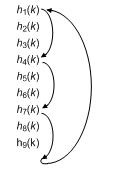
Figure 4: Reduced number of necessary Coefficient Sets, N_D, when decimation
by three is implemented: only three Coefficient Sets
[h₁(k), h₄(k), and h₇(k)] are needed when N=9 and D=3.

In that case we only need to store three Coefficients Sets in memory rather than nine Coefficient Sets.

In the general case for this decimation situation, where where N_D Coefficient Sets are necessary, instead of inputting a single $ x(n) $ sample for each filter output sample computation, we input D $ x(n) $ samples and then proceed to compute a single output sample. And our processing is as shown in Figure 5.

Figure 5: Second-order Translating FIR Filter with decimation
by D using N_D Coefficient Sets.

Another way to view the relationship in Eq. (3) is to accept the following restraint:

$$ \frac {N_DDf_t}{ f_s}= \text{an integer.} \tag{4} $$

Conclusion

We've shown how it's possible to translate a signal down in frequency and lowpass filter in a single operation using a Translating FIR Filter, as shown in Figure 2. We discussed the restrictions on the acceptable f_t translation frequency. This filtering scheme eliminates the cosine multiplier in Figure 1 at the expense of significantly increasing the necessary amount of filter coefficient storage.

It's possible to incorporate filter output decimation (downsampling) in this process, as shown in Figure 5, which reduces the required coefficient storage to a possibly acceptable value. The restrictions on the f_t translation frequency and the decimation factor D are given in Eq. (4).

[This blog was updated on Feb. 12, 2017 based on very helpful comments from Marci Detwiller and Kevin Krieger (University of Saskatchewan).]

References

[1] https://www.dsprelated.com/thread/1567/phase-drift-if-oscillator-doesn-t-go-through-full-360-deg-rotation-when-mixing-fir-to-bandpass

[2] Frerking, M. E., Digital Signal Processing in Communications
    Systems, Chapman & Hall, 1994, pp. 171-174

Appendix A: Why the Figure 2 Filter Works

Here we explain why the Figure 2 Translating FIR Filter works as claimed. Figure A1 shows the traditional scheme for frequency translation followed by lowpass filtering.

Figure A1: Traditional frequency translation
followed by lowpass filtering.

Once the filter's K=6 delay line is filled with data, the $ y(n) $ output sample is equal to:

\begin{eqnarray} y(n) & = & h(0)cos(2 \pi n f_t / f_s)x(n) + h(1)cos[2 \pi (n-1) f_t/f_s]x(n-1) \\ & + & h(2)cos[2 \pi (n-2)  f_t / f_s]x(n-2) + h(3)cos[2 \pi (n-3)  f_t / f_s]x(n-3) \\ & + & h(4)cos[2 \pi (n-4)  f_t / f_s]x(n-4) + h(5)cos[2 \pi (n-5)  f_t / f_s]x(n-5). \tag{A1} \end{eqnarray}

That $ y(n) $ output sample in Eq. (A1) would be the same if we eliminated the initial cosine multiplier altogether and our FIR filter's six coefficients were:

The next $ y(n+1) $  filter output sample is equal to:

\begin{eqnarray} y(n+1) & = & h(0)cos(2 \pi (n+1) f_t / f_s)x(n+1) + h(1)cos[2 \pi (n+1-1) f_t/f_s]x(n+1-1) \\ & + & h(2)cos[2 \pi (n+1-2)  f_t / f_s]x(n+1-2) + h(3)cos[2 \pi (n+1-3)  f_t / f_s]x(n+1-3) \\ & + & h(4)cos[2 \pi (n+1-4)  f_t / f_s]x(n+1-4) + h(5)cos[2 \pi (n+1-5)  f_t / f_s]x(n_1-5). \tag{A2} \end{eqnarray}

For that $ y(n+1) $ output sample a multiplier-free FIR filter's six coefficients would be:

which are different from Coefficient Set# 1. To compute the third $ y(n+3) $ output sample the FIR filter's six coefficients must be:

which are different from Coefficient Set# 1 and Coefficient Set# 2. As such, to eliminate the initial cosine multiplier in Figure A1 we are forced to use a different set of coefficients for each new filter input sample. At first glance this sounds practically impossible to implement! (This situation, what I call "Compute to Extinction", is something to be avoided.)

Here's the good news: if $ f_t $ is an integer submultiple of $ f_s $ then we only need a fixed number of Coefficient Sets because those Coefficient Sets' values repeat.

For example, if the translation frequency is $ f_t = f_s/4 $ then Coefficient Set# 1 would be:

And Coefficient Set# 5 would be

which is equal to Coefficient Set# 1. Coefficient Set# 6 will be equal to Coefficient Set# 2, Coefficient Set# 7 will be equal to Coefficient Set# 3, and so on.

In this scenario, for a simple second-order (each Coefficient Set has three coefficients) FIR filter, our Translating FIR Filter is implemented as shown in Figure A2 with N = 4 unique Coefficient Sets. As each new $ x(n) $ sample arrives to the filter the rotary switches jump to the next Coefficient Set. (After Coefficient Set $ h_4(k) $ is used we switch back to Coefficient Set $ h_1(k) $.) Again, this scheme only works when $ f_t $ is an integer submultiple of $ f_s $.

Figure A2: Coefficient Sets for a second-order lowpass
Translating FIR Filter when f_t = f_s/4.

Appendix B: Important Issues Regarding Translating FIR Filters

• For down-conversion the cosine mixing sequence in Figure 1 would normally be the negative-frequency cosine $ cos(2\pi n [-f_t]/f_s) $ sequence. However, because $ cos(2\pi n [-f_t]/f_s)  = cos(2 \pi n f_t / f_s) $, we'll follow Reference [2]'s convention and use the $ cos(2 \pi n f_t /f_s) $ mixing sequence. 

• The $ f_t $ translation frequency must be an integer submultiple of $ f_s $ to guarantee proper operation in Figure 2. The origin of this restriction is explained in Appendix A.

• Again, the inherent cosine mixing within our Translating FIR Filter translates $ x(n) $ 's spectral components both up and down in frequency. As such, the stopband cutoff frequency of the Figure 1 lowpass FIR filter must be defined so the filter attenuates those higher-frequency spectral components.

• Although the coefficients within any single Coefficient Set are generally not symmetrical, if your original Figure 1 FIR filter is linear phase then the Figure 2 Translating FIR Filter will exhibit linear phase.

• The Translating FIR Filter in Figure 2 is not a linear time-invariant (LTI) system! As such, we cannot determine the filter's frequency response by way performing the discrete Fourier transform (DFT) of the filter's unit impulse response. I suggest using a "swept-frequency input" method to determine the filter's frequency response.

• If the passband gain of the original Figure 1 lowpass FIR filter is G, the passband gain of the Figure 2 filter will be G/2. (That's because mixing with a cosine in Figure 1 reduces the frequency-translated spectral components' peak amplitudes by a factor of two.) To achieve a passband gain of unity for the Figure 2 filter we can merely double the Figure 1 $ h(k) $ coefficients' values or double the amplitude of the mixing cosine sequence.

• Because the coefficients within any single Figure 2 Coefficient Set are generally not symmetrical we typically cannot implement our Figure 2 filter using a folded-FIR filter block diagram in order to reduce the number of multiplies per input sample.

Sign in