


A Two Bin Exact Frequency Formula for a Pure Complex Tone in a DFT
Introduction
This is an article to hopefully give a better understanding to the Discrete Fourier Transform (DFT) by deriving an exact formula for the frequency of a complex tone in a DFT. It is basically a parallel treatment to the real case given in Exact Frequency Formula for a Pure Real Tone in a DFT. Since a real signal is the sum of two complex signals, the frequency formula for a single complex tone signal is a lot less complicated than for the real case.
Theoretical Overview
Similar to the real case, the bin value formula is used on two DFT bins to create a system of two equations (implicitly four, if you count the real and imaginary parts) with three unknowns. A single combination of the two equations eliminates two of the unknowns leaving only the frequency term as unknown. This term is easily isolated and expressed in terms of the known values. From this, the frequency can be calculated. Since the most practical application of this equation will be at the two consecutive bins with the largest magnitude, a special version of the formula is derived for that usage.
A Pure Complex Tone Sequence
A pure complex tone is an exponential function that can be defined by three parameters. The same three as for the real case, they are amplitude ($ M $), frequency ($ f $), and phase ($ \phi $). A discrete pure complex tone is a set of complex signal values within a frame. A frame consists of a defined number of points, $ N $, and the signal values are indexed from $ 0 $ to $ N-1 $. The signal can be extended beyond the frame by using out of range subscripts. Here is an equation defining a pure complex tone: $$ S_n = M e^{i( f \cdot { 2\pi \over N } n + \phi )} \tag 1 $$ The frequency is expressed in units of cycles per frame. For practical purposes the frequency should be constrained to be greater than zero and less than $ N $. It is also possible to use a range of $ -N/2 $ to $ N/2 $. Negative frequencies make a lot more sense for complex tones than for real tones due to the sign determining the chirality of the tone in the time domain. Frequencies outside of the ranges will appear to be frequencies within the range in the DFT. This phenomenon is known as aliasing.
The frequency and bin indexes can be rescaled to a distance along the circumference which is also an angular scale. Defining angle variables makes working with the equations simpler. $$ \alpha = f \cdot { 2\pi \over N } \tag 2 $$ $$ \beta_k = k \cdot { 2\pi \over N } \tag 3 $$ Substituting (2) into (1) gives a simpler formula for the signal. $$ S_n = M \cdot { e^{ i(\alpha n + \phi) } } \tag 4 $$
Bin Value Formula for a Pure Complex Tone
This is a formula to calculate the bin values in a DFT for a pure complex tone: $$ Z_k = { M \over N } e^{ i \phi } \cdot { 1 - e^{ i\alpha N } \over 1 - e^{ i(\alpha - \beta_k ) } } \tag {5} $$ The index $k$ is assumed to range from 0 to $N-1$. The derivation of this formula can be found in my previous blog article titled "DFT Bin Value Formulas for Pure Complex Tones."
Solving for the Frequency Term
For non-integer frequencies a second bin is needed to solve for the frequency. The first bin has the index $ k $ and the second bin has the index $ j $. The formula for the $ j $ bin is the same as that for the $ k $ bin, except $ j $ is substituted for $ k $. $$ Z_j = { M \over N } e^{ i \phi } \cdot { 1 - e^{ i\alpha N } \over 1 - e^{ i(\alpha - \beta_j ) } } \tag {6} $$ (5) can be divided by (6) to give this equation: $$ { Z_k \over Z_j } = { 1 - e^{ i(\alpha - \beta_j ) } \over 1 - e^{ i(\alpha - \beta_k ) } } \tag {7} $$ This operation eliminates $ M $ and $ \phi $, leaving $ \alpha $ as the only unknown. The next step is to cross multiply and separate the exponent terms. $$ Z_k - Z_k e^{ i\alpha } e^{ -i\beta_k } = Z_j - Z_j e^{ i\alpha } e^{ -i\beta_j } \tag {8} $$ The frequency related term $( e^{ i\alpha } )$ occurs twice in the equation. It can be solved for by using ordinary algebra. $$ e^{ i\alpha } = { { Z_k - Z_j } \over { e^{ -i\beta_k } Z_k - e^{ -i\beta_j } Z_j } } = Q_1 \tag {9} $$ The result is that the only unknown is on the left side of the equation and the right side contains known values and can be evaluated.
The Integer Frequency Case
The integer frequency case is a special case where all the DFT bin values will be zero except for the bin value corresponding to the frequency. The formula still works as long as $ Z_k $ or $ Z_j $ is the non-zero bin. If they are both zero, of course the equation won't work. Assuming, without loss of generality, that the $ k $ bin has the non-zero value. It can be seen by inspection that the $ Z_k $ value will cancel out of the numerator and the denominator leaving a negative exponent in the denominator. Flipping the reciprocal means flipping the sign in the exponent leaving $ e^{ i\alpha } = e^{ i\beta_k } $. Thus $ \alpha $ has to be equal to $ \beta $ plus an integer multiple of $ 2 \pi $. Assuming the signal is not an alias, this means $ f = k $. To translate to a negative frequency range, if $ k > N/2 $ then $ f = k - N $.
The Natural Log of a Complex Value
In order to solve for $ \alpha $ in (9) it is necessary to take the natural log of a complex number. To understand what this means it is useful to consider a complex number in both its Cartesian form and its polar form and how the two expressions are related. $$ a + ib = r e^{ i\theta } \tag {10} $$ A point in the complex plane $(a,b)$ corresponds to the complex value $ a + ib $. This representation is unique. It can also be located by the angle from the real axis $( \theta )$ and the distance from the origin $(r)$. This representation is not unique. Any integer multiple of $2\pi$ added to the angle value yields the same angle. The conversion from polar to Cartesian is straightforward trigonometry. $$ a = r \cdot \cos( \theta ) \tag {11} $$ $$ b = r \cdot \sin( \theta ) \tag {12} $$ It follows from Euler's equation: $$ e^{ i\theta } = \cos( \theta ) + i \cdot \sin( \theta ) \tag {13} $$ $$ r e^{ i\theta } = r \cos( \theta ) + i \cdot r \sin( \theta ) = a + ib \tag {14} $$ An explanation, and derivation, of Euler's equation can be found in my first blog article titled "The Exponential Nature of the Complex Unit Circle".
The conversion from Cartesian to polar uses the Pythagorean theorem for the distance to the origin. $$ r = ( a^2 + b^2 )^{ 1/2 } \tag {15} $$ The angle is usually solved for using the Arctangent function. However, this method may require an adjustment of +/- $\pi$ depending upon in what quadrant $(a,b)$ lies. $$ \theta = \tan^{-1} \left( { b \over a } \right) \tag {16} $$ In most math library implementations, there is an alternative function called "atan2". Instead of taking the ratio of $ b/a $ as an argument, it takes $a$ and $b$ as separate arguments. The function properly handles the quadrant adjustments and handles the $a=0$ cases. $$ \theta = \operatorname{ atan2 }( b, a ) \tag {17} $$ The natural log of (10) can now be taken. $$ \ln( a + ib ) = \ln( r ) + i\theta \tag {18} $$ Substituting in (15) and (17) leaves a working definition which uses only $a$ and $b$. $$ \ln( a + ib ) = \ln( a^2 + b^2 ) / 2 + i \cdot \operatorname{ atan2 }( b, a ) \tag {19} $$
Calculating the Frequency
Taking the natural log of (9) leaves this equation: $$ i\alpha = \ln(Q_1) \tag {20} $$ If the bin values correspond to a pure tone the magnitude of $ Q_1 $ will be 1 so the real part of the logarithm will be zero. If the tone's amplitude is growing or decaying exponentially, the rate will be reflected in $ \ln(\|Q_1\|) $, which is the real part of $\ln(Q_1)$. This will be covered in a future blog article.
Since a zero value is expected, the real part of the natural log is discarded and we are left equating the imaginary parts of the logarithm which correspond with the frequency. $$ \alpha = \operatorname{ atan2 }( Im[Q_1], Re[Q_1] ) \tag {21} $$ $Im[Q_1]$ and $Re[Q_1]$ are the imaginary and real parts of $Q_1$. There is an implicit integer multiple of $2\pi$ which can be added to the angle. This accounts for all the alias frequencies that are possible. Converting back from an angle scale to a bin index scale results in the frequency expressed as cycles per frame. The atan2 function will return a value within the range of $-\pi$ to $\pi$, so the frequency will be from $-N/2$ to $N/2$. $$ f = \alpha \cdot { N \over 2\pi } = \operatorname{ atan2 }( Im[Q_1], Re[Q_1] ) \cdot { N \over 2\pi } \tag {22} $$ If a frequency range of 0 to $N$ is desired, negative frequencies can have N added to them. This corresponds to a single $2\pi$ on the angle scale.
Some Numerical Examples
These numerical examples demonstrate the validity of the formula. The source code can be found below in Appendix A. First is a listing of the DFT values and the Roots of Unity used in the DFT calculation and the frequency formula. Following this are three calculations using three different bin pairs. The first pair are the DC bin and the Nyquist bin. The second pair are an arbitrary selection of far apart spaced bins. The third pair are the adjacent bins to the peak value. The calculations are done to a greater precision than the display values.
               DFT                    e^(-i*beta_k)
 k       Real        Imag            Real       Imag
--  --------------------------  --------------------------
 0   0.005657918  0.070641787    1.000000000 -0.000000000
 1  -0.009392193  0.080305352    0.923879533 -0.382683432
 2  -0.030314566  0.093739453    0.707106781 -0.707106781
 3  -0.064623699  0.115769094    0.382683432 -0.923879533
 4  -0.139603486  0.163913062    0.000000000 -1.000000000
 5  -0.500205999  0.395453272   -0.382683432 -0.923879533
 6   0.567743787 -0.290269399   -0.707106781 -0.707106781
 7   0.207141274 -0.058729189   -0.923879533 -0.382683432
 8   0.132161487 -0.010585221   -1.000000000 -0.000000000
 9   0.097852354  0.011444420   -0.923879533  0.382683432
10   0.076929981  0.024878521   -0.707106781  0.707106781
11   0.061879870  0.034542087   -0.382683432  0.923879533
12   0.049722484  0.042348255   -0.000000000  1.000000000
13   0.038948748  0.049265991    0.382683432  0.923879533
14   0.028589040  0.055917882    0.707106781  0.707106781
15   0.017815305  0.062835619    0.923879533  0.382683432

***************************************************
Example Case:   k = 0   j = 8

Num = (0.0057+0.0706i) - (0.1322-0.0106i)
    = (-0.1265+0.0812i)

Den = (1.0000-0.0000i)(0.0057+0.0706i) - (-1.0000-0.0000i)(0.1322-0.0106i)
    = (0.0057+0.0706i) - (-0.1322+0.0106i)
    = (0.1378+0.0601i)

Q1 = Num/Den = (-0.5556+0.8315i)

||Q1|| = 1.0000   Alpha = atan2(Im[Q1],Re[Q1]) = 2.1598

f = Alpha*N/(2Pi) = 5.5000

***************************************************
Example Case:   k = 2   j = 14

Num = (-0.0303+0.0937i) - (0.0286+0.0559i)
    = (-0.0589+0.0378i)

Den = (0.7071-0.7071i)(-0.0303+0.0937i) - (0.7071+0.7071i)(0.0286+0.0559i)
    = (0.0448+0.0877i) - (-0.0193+0.0598i)
    = (0.0642+0.0280i)

Q1 = Num/Den = (-0.5556+0.8315i)

||Q1|| = 1.0000   Alpha = atan2(Im[Q1],Re[Q1]) = 2.1598

f = Alpha*N/(2Pi) = 5.5000

***************************************************
Example Case:   k = 5   j = 6

Num = (-0.5002+0.3955i) - (0.5677-0.2903i)
    = (-1.0679+0.6857i)

Den = (-0.3827-0.9239i)(-0.5002+0.3955i) - (-0.7071-0.7071i)(0.5677-0.2903i)
    = (0.5568+0.3108i) - (-0.6067-0.1962i)
    = (1.1635+0.5070i)

Q1 = Num/Den = (-0.5556+0.8315i)

||Q1|| = 1.0000   Alpha = atan2(Im[Q1],Re[Q1]) = 2.1598

f = Alpha*N/(2Pi) = 5.5000
All the pairs give the same correct exact value for the frequency. In the presence of noise, or other tones, the frequency equation changes from being an exact solution to being an estimator. In those cases, choosing the bin with the largest magnitude and the adjacent one with the next largest magnitude as the pair gives the highest possible accuracy to the result. This not only because the signal to noise ratio is highest in those bins, but also because the bin values are nearly opposite each other making the subtractions in the formula additions of signal information. This can be seen in the numerical examples by judging the magnitudes of the numerator and denominators in the Q1 calculation.
When the Bins are Adjacent
Since the best use of the formula is on adjacent bins, it makes sense to derive a variation for that case. Let $k$ be the lower bin and $j$ be the upper one. $$ j = k + 1 \tag {21} $$ Substituting this into (9) and factoring out a $e^{ -i\beta_k }$ from the denominator leaves this: $$ e^{ i\alpha } = e^{ i\beta_k } { { Z_k - Z_{k+1} } \over { Z_k - e^{ -i\beta_1 } Z_{k+1} } } \tag {22} $$ Both sides can be divided by $e^{ i\beta_k }$ leaving another quotient expression on the right hand side of the equation. $$ e^{ i( \alpha - \beta_k ) } = { { Z_k - Z_{k+1} } \over { Z_k - e^{ -i\beta_1 } Z_{k+1} } } = Q_2 \tag {23} $$ Once again, take the natural log of both sides and discard the real part which will be zero anyway in the pure tone case. $$ \alpha - \beta_k = \operatorname{ atan2 }( Im[Q_2], Re[Q_2] ) \tag {24} $$ Converting back to a bin scale and bringing the base bin index back to the right hand side produces the final version. $$ f = k + \operatorname{ atan2 }( Im[Q_2], Re[Q_2] ) \cdot { N \over 2\pi } \tag {25} $$ The same issues about frequency range and aliases apply to this equation as well. Calculation wise, a complex multiply has been swapped for a real add, so it is marginally more efficient computationally. Because the expected angle from the atan2 function is going to be within a bin width, the Arctangent function can be used instead. This means for certain applications, it may be more efficient to evaluate the first few terms of the Arctangent Taylor series when a good approximation is all that is required.
Conclusion
The derivation of these formulas is not that difficult. The result is a two bin formula for complex tones that is relatively simple. In applications where there is foreknowledge of the approximate frequency of a signal, only the DFT bins in the neighborhood of the frequency need to be calculated.
Appendix A. Source Code Listing
#include <math.h>
#include <stdio.h>

struct complex
{
    double Real;
    double Imag;
};

//============================================================================
void complexProduct( complex* z1, complex* z2, complex* product )
{
        product->Real = z1->Real * z2->Real - z1->Imag * z2->Imag;
        product->Imag = z1->Real * z2->Imag + z1->Imag * z2->Real;
}
//============================================================================
void complexQuotient( complex* z1, complex* z2, complex* quotient )
{
        double den2 = z2->Real * z2->Real + z2->Imag * z2->Imag;

        quotient->Real = ( z1->Real * z2->Real + z1->Imag * z2->Imag ) / den2;
        quotient->Imag = (-z1->Real * z2->Imag + z1->Imag * z2->Real ) / den2;
}
//============================================================================
void showCalcTwoBins( int N, int k, int j, complex* bins, complex* roots )
{
        complex Num, Den, Product_j, Product_k, Q1;

        Num.Real = bins[k].Real - bins[j].Real;
        Num.Imag = bins[k].Imag - bins[j].Imag;

        complexProduct( &roots[k], &bins[k], &Product_k );
        complexProduct( &roots[j], &bins[j], &Product_j );

        Den.Real = Product_k.Real - Product_j.Real;
        Den.Imag = Product_k.Imag - Product_j.Imag;

        complexQuotient( &Num, &Den, &Q1 );

        double Q1_Mag = sqrt(  Q1.Real* Q1.Real + Q1.Imag * Q1.Imag );
        double Alpha = atan2( Q1.Imag, Q1.Real );

        double f = Alpha * N / ( 2.0 * M_PI );

        printf( "\n" );
        printf( "***************************************************\n" );
        printf( "Example Case:   k = %d   j = %d\n", k, j );
        printf( "\n" );

        printf( "Num = (%6.4f%+6.4fi) - (%6.4f%+6.4fi)\n",
                bins[k].Real, bins[k].Imag,
                bins[j].Real, bins[j].Imag );

        printf( "    = (%6.4f%+6.4fi)\n", Num.Real, Num.Imag );

        printf( "\n" );

        printf( "Den = (%6.4f%+6.4fi)(%6.4f%+6.4fi) - (%6.4f%+6.4fi)(%6.4f%+6.4fi)\n",
                roots[k].Real, roots[k].Imag,
                bins[k].Real,  bins[k].Imag,
                roots[j].Real, roots[j].Imag,
                bins[j].Real,  bins[j].Imag );

        printf( "    = (%6.4f%+6.4fi) - (%6.4f%+6.4fi)\n",
                Product_k.Real, Product_k.Imag,
                Product_j.Real, Product_j.Imag );

        printf( "    = (%6.4f%+6.4fi)\n", Den.Real, Den.Imag );

        printf( "\n" );

        printf( "Q1 = Num/Den = (%6.4f%+6.4fi)\n", Q1.Real, Q1.Imag );

        printf( "\n" );

        printf( "||Q1|| = %6.4f   Alpha = atan2(Im[Q1],Re[Q1]) = %6.4f\n",
                Q1_Mag, Alpha );

        printf( "\n" );

        printf( "f = Alpha*N/(2Pi) = %6.4f\n", f );

}
//============================================================================
void DFTbin( int N, int k, complex* signal, complex* roots, complex* result )
{
        complex Product;

        result->Real = 0.0;
        result->Imag = 0.0;

        int nk = 0;

        for( int n = 0; n < N; n++ )
        {
            complexProduct( &signal[n], &roots[nk], &Product );

            result->Real += Product.Real;
            result->Imag += Product.Imag;

            nk += k;
            if( nk >= N ) nk -= N;
        }

        result->Real /= (double) N;
        result->Imag /= (double) N;
}
//============================================================================
int main( int argc, char *argv[] )
{
        int    N    = 16;

        double freq = 5.5;
        double phi  = 1.0;
        double M    = 1.0;

        complex signal[N];

        double alpha = freq * 2.0 * M_PI / (double) N;

        for( int n = 0; n < N; n++ )
        {
            double angle = alpha * (double) n + phi;

            signal[n].Real = M * cos( angle );
            signal[n].Imag = M * sin( angle );
        }

        complex roots[N];

        for( int k = 0; k < N; k++ )
        {
            double beta_k = (double) k * 2.0 * M_PI / (double) N;

            roots[k].Real =  cos( beta_k );
            roots[k].Imag = -sin( beta_k );
        }

        printf( "               DFT                    e^(-i*beta_k)\n" );
        printf( " k       Real        Imag            Real       Imag\n" );
        printf( "--  --------------------------  --------------------------\n" );

        complex bins[N];

        for( int k = 0; k < N; k++ )
        {
            DFTbin( N, k, signal, roots, &bins[k] );

            printf( "%2d  %12.9f %12.9f   %12.9f %12.9f\n",
                    k,
                    bins[k].Real,
                    bins[k].Imag,
                    roots[k].Real,
                    roots[k].Imag );
        }

        showCalcTwoBins( N, 0,  8, bins, roots );
        showCalcTwoBins( N, 2, 14, bins, roots );
        showCalcTwoBins( N, 5,  6, bins, roots );

        return 0;
}
//============================================================================
- Comments
- Write a Comment Select to add a comment

Hi. It seems to me that your blog falls under the topic called "frequency estimation." This topic has been studied for over 20 years producing dozens of different algorithms to estimate frequency based on DFT sample values; such as the Parabolic method, Jacobsen/Kootsookos methods, Quinn's estimator, Jain's method, Lyons' method, Grandke's method, Candan's method, to name just a few.
In fact, there's an entire book covering this 'frequency estimation' topic:
https://www.amazon.com/Improving-Frequency-Resolution-Discrete-Spectra/dp/3838359437
Cedron Dawg, I wonder how well your Eqs. (23) and (25) perform (accuracy-wise) compared to previously published frequency estimation methods. Perhaps the following paper by Jacobsen & Kootsookos would be of interest to you:
http://citeseerx.ist.psu.edu/viewdoc/download?doi=10.1.1.555.2873&rep=rep1&type=pdf

Hi Rick,
It sure does. I am familiar with J & K's paper and I can tell you all those methods are approximation equations, meaning they don't get the correct answer in the noiseless case. I believe the term for this is "biased". In contrast, my equations are exact. In the presence of noise both sets become estimators. I like to make the distinction between an estimator which is an equation that does as well as it can in the absence of full information (e.g. knowing the noise) versus an approximation which is an equation that usually had some simplifying assumptions made during its derivation.
Out of all the methods you mentioned, only Candan's 2013 formula is exact. You wouldn't know that from his derivation. I know it because I figured out mathematically that it was equivalent to my three bin formula which I know is exact. I was perplexed why his numbers and mine were nearly identical in the testing.
Both of those formulas can be found in Julien Arzi's excellent frequency equation comparison report which can be found here:
http://www.tsdconseil.fr/log/scriptscilab/festim/i...
I have previously published results for the complex signal case in comp.dsp. You can find them here:
https://www.dsprelated.com/showthread/comp.dsp/278...
I did misstate Candan's formula there. It should be
f = k + atan( Real( q ) tan(Pi/N) ) / (Pi/N).
You can see from the results that the 2 bin formula significantly outperforms the 3 bin formulas. This is due to the third bin having a much lower SNR compared to the two larger bins. This advantage only disappears when the frequency gets close to an integer and the third bin has roughly the same SNR as the smaller second bin and thus its contribution becomes more valuable.
I have a few more exact formulas to present, then I'm going to write a blog article showing the results for all of them.
The irony is that I have been told many "experts" that exact formulas are impossible. I think I have proved them wrong.
If you have the book you cited, perhaps you can tell me if it claims any of its formulas are exact.
Ced
Hi Cedron. What I've seen in the past is that most of the freq estimation algorithm's have a small fixed-bias error when the input sinusoid is noise-free. Grandke's method has a SUPER-small bias error when the input sinusoid is noise-free. However, when the input sinusoid is contaminated with noise (say SNR = 9 dB) Jacobsen's method appears to have the smallest mean error and an error variance similar to the other methods. By "Jacobsen's method" I mean Eq. (3) at:
http://citeseerx.ist.psu.edu/viewdoc/download?doi=10.1.1.555.2873&rep=rep1&type=pdf
In my testing, in the presence of noise Jacobsen's method is superior to Grandke's essentially bias-free algorithm. What that tells me is that testing a freq estimation algorithm with noise-free input sinusoids is not a valid test.
I think the best way to gauge the value of a freq estimation algorithm is to:
(1) Input a noisy sinusoid whose frequency sweeps from one DFT bin center to the next higher DFT bin center.
(2) Measure the algorithm's freq estimation error at various freqs between one bin center and the next bin center.
(3) Repeat Steps (1) & (2) 100 or a 1000 times and compile statistical data on the variance of the errors (versus frequency) and the mean of the errors (versus frequency).
With that statistical data you're then able to compare the performance of two different freq estimation methods is a realistic way.
(By the way, I do not have a copy of the Gasior book.)
Hi Rick,
I don't have Grandke's formula coded, but since it is worse than Jacobsen's in noise that shouldn't matter.
You're testing methodology is a very accurate description of what I did in the comp.dsp thread referenced above, and my current testing.
By "sinusoid" I assume you mean "complex sinusoid", that is we are currently talking about complex signals.
Here is a preview of my results blog article, tailored specifically for your request. The first column is the mean of the error (x100) and the second column is the standard deviation (x100). I prefer the std dev over the variance because it is on the same scale.
The target noise level is the std dev of the noise. The amplitude of the signal is 1. I believe I have the correct value for a SNR of 9 dB.
The results for my 3 bin complex formula and Candan's 2013 are identical since they are mathematically equivalent, so I have combined them into one display set.
Notice that the std dev for Candan's and Jacobsen's are nearly identical because Candan's is Jacobsen's with a correction term. Jacobsen's inherent bias shows up in the noiseless case whereas my two bin and three bin (and Candan's) are exact so there is no error.
Also notice that the two bin does better between the bins and the three bin does better near the integer frequencies as I mentioned above.
Ced
The sample count is 100
and the run size is 100
Errors are shown at 100x actual value
Target Noise Level = 0.000
Freq CD2Bin CD3Bin/Candan Jacobsen
---- ------------- ------------- -------------
3.0 0.000 0.000 -0.000 0.000 -0.000 0.000
3.1 0.000 0.000 -0.000 0.000 -0.003 0.000
3.2 0.000 0.000 0.000 0.000 -0.006 0.000
3.3 0.000 0.000 0.000 0.000 -0.009 0.000
3.4 0.000 0.000 0.000 0.000 -0.011 0.000
3.5 -0.000 0.000 0.000 0.000 -0.012 0.000
3.6 -0.000 0.000 0.000 0.000 0.011 0.000
3.7 0.000 0.000 -0.000 0.000 0.009 0.000
3.8 0.000 0.000 0.000 0.000 0.006 0.000
3.9 -0.000 0.000 0.000 0.000 0.003 0.000
Target Noise Level = 0.355
Freq CD2Bin CD3Bin/Candan Jacobsen
---- ------------- ------------- -------------
3.0 0.221 2.731 0.054 1.963 0.054 1.962
3.1 -0.255 1.810 0.049 1.988 0.046 1.987
3.2 0.480 1.649 0.171 1.976 0.164 1.976
3.3 0.171 1.460 0.199 2.164 0.190 2.163
3.4 -0.101 1.334 -0.382 2.397 -0.393 2.396
3.5 -0.046 1.477 0.182 3.021 0.169 3.021
3.6 -0.057 1.330 0.192 2.700 0.203 2.700
3.7 -0.188 1.353 -0.239 1.931 -0.230 1.931
3.8 -0.014 1.674 -0.253 2.145 -0.247 2.145
3.9 0.041 2.190 -0.002 1.690 0.002 1.690
Hi. You call your freq estimation method "exact." Now I don't know what "exact" means but I mention Grandke's method because I THINK you would also call Grandke's method "exact." If I'm correct, then I mentioned Grandke's method to show that a so-called "exact" method may not work too well with noisy input signals.
Cedron, I'm not smart enough to make sense out of your lists of numbers. If you could plot various freq estimation methods' error variance and mean error in 2-dimensional plots (where the x-axis is frequency from one DFT bin center to the next DFT bin center) then I'd be better able to evaluate their performances. (Who is it that said, "A picture is worth a thousand words"?)
Hi Rick,
"Exact" has a very strong definition in mathematics. Basically it means precise to an infinite number of decimal places.
Grandke's method is not exact. He makes an approximation to produce his equations (9a) and (9b). Also the results in Table 1 show that his method is not exact. (1983 Paper)
I don't dispute that exact solutions may perform poorly in the presence of noise. This is true of the magnitude and phase equations that can be derived in a manner similar to the way I derived the frequency formula. This is why I provide a different method in my blog article "Phase and Amplitude Calculation for a Pure Real Tone in a DFT: Method 1" for real tones, and I will be writing a similar, simpler one, for complex tones.
As my numbers show, the frequency formula is quite robust in the presence of noise. I urge you to code it yourself in some of your test code. It is not that complicated of a formula.
I want to emphasize that there was no interpolation function, or peak thereof, used in the derivation of the frequency formula. Instead, equation (5) matches the values of the Dirichlet kernel (convolved with the signal) at the bins, but not in between. Since it is a simpler function, it is possible to combine two bins worth and solve for the frequency of the tone. This is why I derived the formula first for any two arbitrary bins and then did the adjacent bins second.
Perhaps I will include some graphs when I write up the article. For now let me try to explain the numbers again. For the noiseless case, only the first column under each header matter because the standard deviation column will always be zero for all estimators. The first column is the mean (or arithmetic average) of the error (calculated frequency - actual frequency) * 100. Since CD2Bin and CD3Bin/Candan are exact they have zeroes in this column. Note that the converse isn't necessarily going to be true. Jacobsen's does not, it is biased. In the noisy case, the first column (the mean) is largely a matter of chance and aren't that important. Although you can see for the Jacobsen case, the bias is still there. The second column is the standard deviation which is merely the square root of variance. So if the std dev is bigger than the variance is too. The standard deviation measures the spread of the error distribution so smaller is better.
For the CD2Bin case, the graph looks like a concave upward parabola centered at 3.5. For the other two, it looks like a concave downward parabola also centered and peaking at 3.5. The two parabolas intersect somewhere around 3.15 and 3.85 roughly speaking. In between these two values the two bin performs better and outside this range, that is near integer frequencies the three bin performs better.
I really recommend that you (and everybody) carefully review the derivation of (5) from the prior blog article so you understand where it came from. Then study (6) through (9) to see how two bins are used to solve for the frequency.
Once you "get it", you can go back to my blog articles concerning the real tone case and understand why they are exact too. They are more complicated, but the methodology is basically the same.
Ced
Here is a run of 10,000.
Target Noise Level = 0.355Freq CD2Bin CD3Bin/Candan Jacobsen
---- ------------- ------------- -------------
3.0 -0.051 2.526 -0.021 1.770 -0.021 1.769
3.1 -0.029 2.105 -0.029 1.829 -0.032 1.829
3.2 -0.011 1.777 0.004 1.949 -0.002 1.948
3.3 0.004 1.559 0.003 2.124 -0.005 2.124
3.4 0.001 1.440 -0.011 2.416 -0.022 2.416
3.5 -0.004 1.397 -0.027 2.754 -0.039 2.754
3.6 0.001 1.456 -0.042 2.441 -0.031 2.441
3.7 -0.008 1.582 0.017 2.134 0.026 2.134
3.8 0.006 1.765 0.006 1.943 0.013 1.942
3.9 0.033 2.089 0.023 1.819 0.026 1.818
Here is another run of 10,000 with better headers and more frequency values.
Remember that the values shown are 100x the actual values.
Ced
Target Noise Level = 0.355
Freq CD2Bin CD3Bin/Candan Jacobsen
Mean StdDev Mean StdDev Mean StdDev
---- ------------- ------------- -------------
3.00 -0.023 2.527 -0.009 1.775 -0.009 1.774
3.05 -0.010 2.300 0.005 1.803 0.004 1.803
3.10 0.003 2.096 0.014 1.828 0.011 1.827
3.15 -0.017 1.924 -0.025 1.861 -0.029 1.860
3.20 -0.044 1.767 -0.041 1.929 -0.047 1.929
3.25 0.018 1.653 -0.000 2.028 -0.008 2.028
3.30 -0.013 1.566 -0.022 2.122 -0.031 2.121
3.35 0.008 1.484 0.001 2.256 -0.009 2.255
3.40 0.030 1.451 0.022 2.413 0.011 2.413
3.45 -0.004 1.411 0.011 2.578 -0.001 2.578
3.50 0.026 1.408 0.019 2.813 0.007 2.813
3.55 0.012 1.408 0.009 2.612 0.021 2.612
3.60 -0.003 1.447 0.003 2.444 0.014 2.444
3.65 0.016 1.494 0.022 2.238 0.032 2.237
3.70 0.003 1.572 0.011 2.130 0.020 2.130
3.75 0.026 1.664 0.021 1.988 0.029 1.987
3.80 -0.011 1.791 -0.018 1.977 -0.011 1.976
3.85 -0.001 1.923 -0.014 1.891 -0.009 1.890
3.90 0.002 2.106 0.016 1.837 0.019 1.837
3.95 0.017 2.299 -0.010 1.800 -0.009 1.799
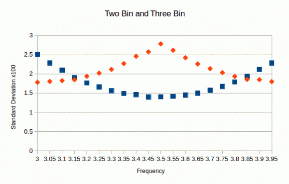
Here is a quick and dirty graph made with a spreadsheet program. It seems I was a little off in my previous description. The three bin case is also an concave upward parabola-like centered at the bin values.
Clearly the two bin is better (lower) for most of the frequencies, the break evens are roughly at 3.15 and 3.85 as I said earlier.
Ced
To post reply to a comment, click on the 'reply' button attached to each comment. To post a new comment (not a reply to a comment) check out the 'Write a Comment' tab at the top of the comments.
Please login (on the right) if you already have an account on this platform.
Otherwise, please use this form to register (free) an join one of the largest online community for Electrical/Embedded/DSP/FPGA/ML engineers:


