


Above-Average Smoothing of Impulsive Noise
In this blog I show a neat noise reduction scheme that has the high-frequency noise reduction behavior of a traditional moving average process but with much better impulsive-noise suppression.
In practice we may be required to make precise measurements in the presence of highly-impulsive noise. Without some sort of analog signal conditioning, or digital signal processing, it can be difficult to obtain stable and repeatable, measurements. This impulsive-noise smoothing trick, originally developed to detect microampere changes in milliampere signals, describes a smoothing algorithm that improves the repeatability of signal amplitude measurements in the presence of impulsive noise[1].
Traditional Moving Average
Practical noise reduction methods often involve an N-point moving-average process performed on a sequence of measured x(n) values, to compute a sequence of N-sample arithmetic means, M(q). As such, the moving-average sequence M(q) is defined by:
$$ M(q) = \frac{1}{N} \sum_{k=q}^{q+(N-1)} x(k) \tag{1} $$
where the time index of this averaging process is q = 0,1,2,3, ... .
The Smoothing Algorithm
The proposed impulsive-noise smoothing algorithm is implemented as follows: collect N samples of an x(n) input sequence and compute the arithmetic mean, M(q), of the N samples. Each sample in the block is then compared to the mean. The direction of each x(n) sample relative to the mean (greater than, or less than) is accumulated, as well as the cumulative magnitude of the deviation of the samples in one direction (which, by definition of the mean, equals that of the other direction). This data is used to compute a correction term that is added to the M(q) mean according to the following formula:
$$ A(q) = M(q) + \frac{(P_{os}-N_{eg}) \cdot \lvert D_{total} \rvert }{N^2} \tag{2}$$
Variable A(q) is the corrected mean, M(q) is the arithmetic mean (average) from Eq. (1), Pos is the number of samples greater than M(q), and Neg is the number of samples less than M(q). Variable Dtotal is the sum of deviations from the mean (absolute values and one direction only). Variable |Dtotal,| then, is the magnitude of the sum of the differences between the Pos samples and M(q). A more detailed description of |Dtotal| is given in Appendix A.
For a simple example, consider a system acquiring 10 measured samples of 10, 10, 11, 9, 10, 10, 13, 10, 10, and 10. The mean is M = 10.3, the total number of samples positive is Pos = 2, and the total number of samples negative is Neg = 8 (so Pos‑Neg = ‑6). The total deviation in either direction from the mean is 3.4 [using the eight samples less than the mean, (10.3‑10) times 7 plus (10.3‑9); or using the two samples greater than the mean, (13‑10.3) plus (11‑10.3)]. With Dtotal = 3.4, Eq. (2) yields the "smoothed" result of A = 10.096.
The Eq. (2) smoothing algorithm's performance, relative to traditional moving-averaging, can be illustrated by a more realistic example. Figure 1(a) shows a measured 500-sample x(n) input signal sequence comprising a step signal of amplitude one contaminated with random noise and three large impulsive-noise spike samples.
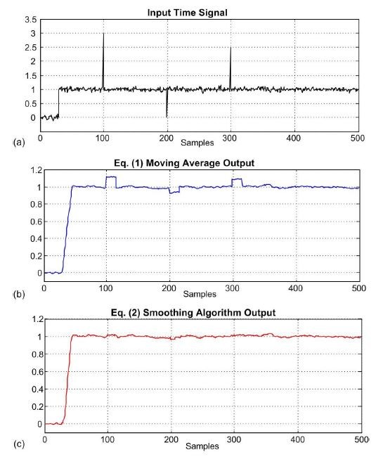
Figure 1: Impulsive
noise smoothing for
N = 16: (a) input
x(n)
signal;
(b)
moving average output; (c) smoothing
algorithm output.
Figure 1(b) shows the Eq. (1) moving average output while Figure 1(c) shows the Eq. (2) smoothing algorithm's output.
We compare the outputs of the moving average and smoothing algorithms in a more concise way in Figure 2. There we see that the input x(n)'s high-frequency noise has been reduced in amplitude by the Eq. (2) smoothing algorithm (in a way very similar to moving averaging) but the large unwanted impulses in Figure 1(a) have been significantly reduced at the output of the Eq. (2) smoothing algorithm.
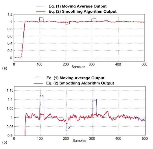
Figure 2: Comparison of the moving average and smoothing algorithm outputs.
If
computational speed is important to you, notice in Eq. (2) that if
N is an integer power of two then the
compute-intensive division operation can be accomplished by binary arithmetic
right shifts to reduce the computational workload.

References
[1] Dvorak, R. “Software Filter Boosts Signal-Measurement Stability, Precision,” Electronic Design Magazine, February 3, 2003.
Appendix A: Definition of |Dtotal|
The definition of the variable |Dtotal|, for a given sequence, can be illustrated with a simple example. have a look at the simple 8-sample x(n) sequence in Figure A-1(a) whose mean (average) is M = 5.19, where
$$ M = \frac{1}{8} \sum_{n=0}^7 x(n) \tag{A-1}$$
For this x(n)
input, five samples are greater than
M
and three samples are less than M.
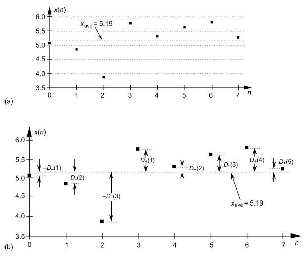
Figure A1: Values used to compute |Dtotal| for the example x(n) sequence.
For the sequence x(n) the variable |Dtotal| is the absolute value of the sum of positive deviations from M, |D+(1)+D+(2)+D+(3)+D+(4)+D+(5)|, as shown in Figure A1(b). And the nature of the arithmetic mean given in Eq. (A-1) is such that variable |Dtotal| is also equal to the absolute value of the sum of negative deviations from M, |D-(1)+D-(2)+D-(3)|. So we can express variable |Dtotal| as:$$ \lvert D_{total} \rvert = \lvert D_+(1) + D_+(2) + D_+(3) + D_+(4) + D_+(5) \rvert $$ $$ = \lvert D_-(1) + D_-(2) + D_-(3) \rvert \tag{A-2}$$
- Comments
- Write a Comment Select to add a comment

Rick
Any idea how this smoother might compare with a N-point median filter? Thanks, for all the books and ideas that you have shared with the community over the years!
Wayne

With my simple test signals, constant amplitude signals contaminated with wideband random noise and occassional unwanted narrow impulsive amplitude spikes, I found that the proposed scheme and median filtering (median smoothing) produced VERY similar results. The two smoothing schemes reduced the unwanted impulsive noise to a very similar degree and the variances of the two schemes' outputs were VERY similar. So I'll "stick my neck out" and say, "It appears to me that there's no significant performance difference between the proposed smoothing scheme and your every-day garden-variety median filtering."
Wayne, your question illustrates my laziness. What I didn't do is compare the computational workload of the proposed smoothing scheme to the computational workload of median filtering. :-(
Rick
There are many whom I might call lazy but you are not one of them! I have learned a great deal from your books over the years. Writing clear English prose is often harder than writing code.
My very dog eared copy of "Understanding Digital Signal Processing (third edition) bears witness to your efforts.
Thanks for your insights concerning this filtering scheme. The filter is not hard to implement, I might do my own comparison between a median filter and your smoother.
Wayne
Hi Wayne.
Thanks again. I can send you the errata for the 3rd edition of my "Understanding DSP" book. If you're interested, send my a private e-mail at:
R.Lyons@ieee.org
Wayne, if you model the two smoothing schemes I'd be interested to learn about your modeling results.

On behalf of Wayne (and by the way it is first time I see his posts) I did the following matlab modelling and you can see the median is far more powerful on (single isolated) spikes. I hope I done it right
*******************************************
x = randn(1,1024);
x(36) = 17; x(178) = -20; x(455) = -33;
p = 0; n = 0; s = 0;
for i = 1+10:1024
m(i) = mean(x(i-10:i));
if x(i) > m(i),
p = p+1;
s = s + x(i);
elseif x(i) < m(i),
n = n + 1;
end
m(i) = m(i) + (p - n)*s/i^2;
test(i) = median(x(i-10:i));
end
plot(m);hold;
plot(test,'r--');
******************************
s = s + x(i);
should be: s = s + x(i) -m(i);
Also, I think your command:
m(i) = m(i) + (p - n)*s/i^2;
should be: m(i) = m(i) + (p - n)*s/11^2;
where the denominator of the second term is eleven squared. (That denominator must be a constant.)
However, when I make those changes to your MATLAB code my "proposed smoothing" computational results are obviously incorrect. So Kaz, ...I haven't yet figured out what's going on here, but I'm still working on it.
Hi Rick,
Your first correction of:
s = s + x(i) -m(i);
is ok but second one is wrong as it should be I^2 (i.e. N^2) since filter is in running mode.
I can see why median filter is more potent for spikes as it totally ignores peaks if peaks with other samples fall within the taps segment while your formula gives weight to every sample.
Hi Kaz. I'm not sure what your last reply's variable 'I' (uppercase 'i') is. In your code:
when i = 11, you process samples x(1) -to- x(11),
when i = 12, you process samples x(2) -to- x(12),
when i = 13, you process samples x(3) -to- x(13), and so on.
So your value for 'N' in my blog's Eq. (2) is: N = 11. And that's why I said I thought your command:
m(i) = m(i) + (p - n)*s/i^2;
should be: m(i) = m(i) + (p - n)*s/11^2; where the denominator of the second term is eleven squared.
I think for each new value of your loop counter 'i' you need to reset variables 'p', 'n', and 's' to zero. I say that because, for example when N = 11 the maximum value for 'p' can never be greater than 10. But your maximum value for 'p' often increases in value to be greater than 500!
Hi Rick (and Kaz),
You are correct.
I tried the code from Kaz, but I included a small function to reset 'p', 'n', and 's' to zero. It worked ok. In fact, seems like it improves the median filter. I've also changed "I" to "N". Here is the code:
**********************************
x = 5+randn(1,1024);
x(36) = 17; x(178) = -20; x(455) = -33;
L=length(x);
N=10;
p = 0; n = 0; s = 0; s2=0;
for i = N+1:L
m(i) = mean(x(i-N:i));
[s,p,n]=Dtotal(m(i),x(i-N:i));
m(i) = m(i) + (p - n)*s/N^2;
test(i) = median(x(i-N:i));
end
subplot(2,1,1)
plot(m,'b-');hold;
plot(test,'r--');
title("Smoothers")
legend('AboveAverage','meanfilter')
subplot(2,1,2)
plot(x,'k')
title("original")
******************************
The function is:
+++++++++++++++++++++++++++++++
function [s,p,n]=Dtotal(m,x)
p = 0; n = 0; s = 0;
for i=1:length(x)
if x(i) > m,
s = s + x(i)-m;
p = p+1;
elseif x(i) < m,
n = n + 1;
end
end
endfunction
+++++++++++++++++++++++++++++
Sorry if this is too simple, but I had to try it :)
Thanks gmiram. Model now looks ok to me. I added more spikes as below and it does seem that Rick's algorithm is better than median but not so if dc = 0.
%%%%%%%%%%%%%%%%%%
x = 5*0+randn(1,2^14);
x(36:100:end) = 17; x(178:200:end) = -20; x(455:50:end) = -33;
%%%%%%%%%%%%%%%%%
and the rest of code is same as yours above
Hi Kaz. That's a clever way to add multiple impulses. Neat!!
Hi gmiram. Your code looks correct to me (except I think the legend title: "meanfilter" should be "median filter"). Thanks for posting your code.
Sure!
that should say "median filter".
Thanks.
As I read through the description of the filter, I came to the conclusion that it must actually be a "conceptually easy" way to estimate the median. It would be interesting to develop the math to compare them and compute the error, but I'll leave that work to someone else :-).
I think this approach offers some smoothing whereas the median tends to stick to the quantum levels of the original inputs (or a half-way point between them). It would also be interesting to compare computational load -- and for that, I'm guessing the most efficient way to keep track of median across a sliding window would be by managing two heaps: a min-heap for the values above median and a max-heap for the values below median. I've implemented such a thing before -- its a nice exercise, and the resulting data structure is probably about as efficient as you can get for the job. My first guess is that computing the median that way (with the heaps) would require fewer comparisons at each advance of the window. But I still like the idea of what this median-estimate can do.
Of course, another filter type to compare is the LULU, and I've found that combining different sizes can give good results (like averaging the results of a 5x3 and and a 3x5 for a small-ish window size) -- I expect LULU is similar to this approach in terms of computational load.
Hello zimbot.
What does "LULU" mean?
[-Rick-]
Think of it as "lower" and "upper". You take a neighborhood, break it into so many chunks of a given size, take the max and min of each chunk, then get the max of the mins and the min of the maxes. You can average those two values or something even more clever with them. There's a nice overview on wikipedia of Lulu smoothing.
Hi Rick,
This algorithm is amazing. This helped in comparing the running average filter for my application.
Could this algorithm be extended for specific cutoff frequency by adjusting the window size or any other parameters. This could be interesting if you have any further comments regarding this.
Pranav
Hi Yottabyte. Regarding the proposed smoothing technique, the only other comments I have are the following:
[1] That larger the magnitude of the unwanted impulses, the larger must be 'N' to achieve a given amount of impulse smoothing.
[2] The wider in time (measured in samples) are the unwanted impulses, the larger must be 'N' to achieve a given amount of impulse smoothing.
[3] Although my statistical analysis comparing the outputs of a traditional median filter and the proposed smoothing filter is correct, that analysis doesn't indicate what I've noticed to be a performance difference between those two smoothing techniques. Follow-on experimentation leads me to believe that median filtering is superior to the smoothing scheme I've described in this blog.
[4] Again, I have not compared the computational workload (arithmetic operations per output sample) of the
proposed smoothing scheme to the computational workload of median
filtering. :-(
Hi Rick,
Thank you for the comments. However as an observation from my results, there is always an inherent time delay which increases larger the N.
Pranav
Hi Pranav,
you can use impulse input for x, get output from above code and do fft to study frequency response such as cutoff, attenuation etc.
Hi Kaz,
Ya! That would give more details.
Pranav
Hi Rick
Thanks to your skillful and practical idea
I had a question. The idea of implementing it was much better than Translation Invariant Wavelet Denoising
Is there any difference in noise removal with this method?
Hello kafshvandi. I must tell you that the proposed impulsive-noise reduction scheme described in my blog is not my idea. I learned of that scheme from the Reference given in my blog.
I hate to admit it but I have never heard of the "Translation Invariant Wavelet Denoising" method before. Being almost totally ignorant of wavelet transforms, sadly, I'm unable to answer your question. Sorry about that.
Thanks for sharing.
To post reply to a comment, click on the 'reply' button attached to each comment. To post a new comment (not a reply to a comment) check out the 'Write a Comment' tab at the top of the comments.
Please login (on the right) if you already have an account on this platform.
Otherwise, please use this form to register (free) an join one of the largest online community for Electrical/Embedded/DSP/FPGA/ML engineers:


