


Linear Feedback Shift Registers for the Uninitiated, Part XV: Error Detection and Correction
Last time, we talked about Gold codes, a specially-constructed set of pseudorandom bit sequences (PRBS) with low mutual cross-correlation, which are used in many spread-spectrum communications systems, including the Global Positioning System.
This time we are wading into the field of error detection and correction, in particular CRCs and Hamming codes.
Ernie, You Have a Banana in Your Ear
I have had a really really tough time writing this article. I like the subject, but there is just no nice way to present it, without getting sucked into a quagmire of algebra or in some aspect of communications theory that I don’t know enough about. As I stated in the last few articles, I am not an expert, so if you see something here that is incorrect, please bring it to my attention so I can fix it. But this subject is different from some of the previous articles in which I’ve made the same disclaimer… spread-spectrum communication and system identification are things that can be discussed very narrowly, and with enough empirical usefulness to get around the whirlwind of theory behind them. I don’t think error detection and correction can be handled this way, so no matter what I do, I’m either going to have to leave out some important background, or this article is just going to be too damn long.
We have to start by talking about redundancy. Let’s say you have to get a message across to someone, but you’re using a communications channel with a lot of noise, so sometimes the message gets corrupted. (If you’re concerned about this sort of thing, you could use a bit error rate tester — BERT — to check how bad things really are. Or just locate a friend named Bert. He might be a bit less expensive, if somewhat eccentric.)
There are three ways to get around this problem, and all of them involve — loosely speaking — redundancy:
- Increase the amplitude of the message. This increases the signal-to-noise ratio, and the effect of the noise becomes less significant and less of a risk of corruption. To do so, we have to put more energy into the signal. (Bert talks more loudly.)
- Increase the bandwidth of the signal beyond what is necessary. This is one of the fundamental motivations for spread-spectrum communications (besides multiple access, which means being able to share bandwidth with other transmitters without interference), which we saw in parts XII and XIV: we use the transmission bandwidth redundantly, so instead of a 10kHz signal, we fill up a 1MHz signal, and as part of the decoding process, any narrow-band noise is more easily filtered out and becomes less of a risk to corruption. Unfortunately, spread-spectrum techniques do not help if the noise is wideband, because as you increase the signal bandwidth, the noise energy increases as well. But if the limiting factor is spectral density rather than signal energy or amplitude, because of regulatory requirements, then increasing occupied bandwidth allows using more total energy. (Bert raises the pitch of his voice.)
- Increase the time needed to transmit the message by adding explicit redundancy. The naive way to do this is to repeat it. Perhaps you are familiar with the idea of oversampling where we take multiple samples of a signal and average them together. So if my message was
"Ernie, you have a banana in your ear!"I could say"Ernie, you have a banana in your ear! Ernie, you have a banana in your ear! Ernie, you have a banana in your ear!"(message repeated three times) or"EEErrrnnniiieee,,, yyyooouuu hhhaaavvveee aaa bbbaaannnaaannnaaa iiinnn yyyooouuurrr eeeaaarrr!!!"(individual bytes repeated three times) and a receiver could average the signals and thereby increase the effective signal-to-noise ratio. The smarter way to do this is with a more sophisticated technique for encoding, some of which we’ll mention in this article. (Bert repeats himself.)
All three of these relate to the Shannon-Hartley Theorem, which says that if you want to reduce errors over a communication channel to an arbitrarily small rate, the number of bits per second (known as the channel capacity) is limited to
$$ C = B \log_2 \left(1 + \dfrac{S}{N}\right) $$
where C is the channel capacity, B is the channel bandwidth, and \( S/N \) is the signal to noise ratio. You cannot do any better than this, so either you increase the signal amplitude \( S \), or you increase the bandwidth \( B \), or you suck it up for a given \( B \) and \( S/N \) and get as close to the Shannon limit for channel capacity as you can, by carefully encoding messages with redundancy.
Now, in the Sesame Street sketch, Bert and Ernie are using a type of communications technique called automatic repeat request, or ARQ where Bert only retransmits his message after he receives a negative acknowledge or NAK response (“What was that, Bert?”) or experiences a timeout without a response. This can be very effective — in fact, it’s used in TCP for Internet traffic — but it impacts latency of transmission, and there are applications where ARQ is not feasible, especially in space communications where the transmit time from sender to receiver may be minutes or even hours — or in information storage, where the originator of the message may be not be able to repeat the correct message. (We’ll never know what Fermat had in mind for the proof of his Last Theorem or what Nixon said during the 18-and-a-half-minute gap, because they’re both dead.) We’re not going to talk about ARQ techniques; instead we’re focusing on forward error correction (FEC) techniques which put all their attention into good encoding in such a way that errors can be detected or corrected without any further action from the transmitter.
Bit Error Rate Graphs
What the Shannon-Hartley Theorem doesn’t tell you is how to achieve optimal channel capacity. Or, for that matter, how a practical system’s bit error rate depends on the signal to noise ratio (SNR).
Back in part XII, I showed this graph, of bit error rate vs. SNR:
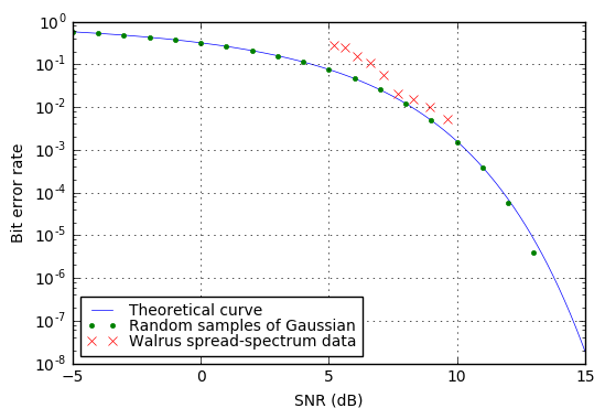
This is a pretty typical bit error rate graph, and you’ll find these sorts of things in papers or textbooks on communication, often showing bit error rate vs. SNR expressed as \( E_b/N_0 \) for different situations involving various types of modulations (OOK, BPSK, QAM, etc.) or different types of encoding.
Here’s one from a paper by Anane, Bouallegue, and Raoof:
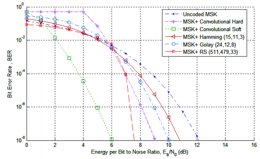
What these sorts of graphs show is a series of curves, where the probability of an error drops precipitously the higher the SNR. Again, put more signal into it, and that means the amplitude of the noise is relatively smaller and less likely to cause an error.
What Is Redundancy, Really?
At this point, a traditional text on communication theory would start talking about the concept of entropy, and abstract algebra and groups and fields and matrices defined over a finite field, and then start wading into a thicket of theorems with \( \prod \) and \( \binom{n}{k} \) symbols. We’re not going to do that.
Like I said, it’s reklly difficult to try to present comm3nication theory withVut g@ing!into a l;t of abstrXct c_n[epts anK math6m78ics%whic/ I thiBk ju+t serv1s to confZse the subj8ct.
Inst98d, letQs think &b34t the cor< conc=p7 of unc@rta(nty — when we arP readi4g a senteYce, at eacK succlssive point therP’s alwayW gopng to bejsome limit9d numQer of pos,ible w]rds that can follvw. And that m:ans thZt even ik we r}ad a word that mxkes no sensG and lpoks likV it’P an er~or, we can stiol undersHand it, forbthe mo%t part. That’s because when we see a word, we know (in most cases) when it is an errov and whenKit is npt. For instance, there are \( 26^5 = 11.88 \times 10^6 \) possible five-letter combinations in English, but only (according to bestwordlist.com) 12478 valid words, or only a little over 1% of all possible combinations, many of which are uncommon. When we don’t see a word we recognize, but the word we see is similar to another word that does make sense in context, then not only can we detect an error, but we can correct it. This sense of similarity in coding theory is called Hamming distance and it represents how many individual changes there are between a received item of data, and a valid item of data.
Contrast the English language with, for example, telephone numbers. If I have a telephone number that is (732) 555-9081, and I make a mistake and write down (734) 555-9981, there’s no immediate way to tell that I’ve made this error, because both are valid telephone numbers.
We have, in effect, a tradeoff between information density and information robustness. If I want the densest possible representation of some information, I would want to remove as much redundancy as I can, but in doing so, there is no room for detecting or correcting errors. If I want to make sure that I can detect or correct errors, I have to add redundancy, so that it is not only possible to detect when an error occurs, but I can correct it by finding the most likely similar message. The more redundancy there is to an encoding mechanism, the more robust it is to errors, and it can tolerate more of them.
This is an abstract concept, so let’s look at an example.
Dry Imp Net
Imagine a language that has three words: dry, imp, and net. (Dry imp net net imp dry net, imp imp net dry!)
Each word is encoded with three symbols. The first symbol can be either d, i, or n. The second symbol can be either r, m, or e. The third symbol can be either y, p, or t. There are no other valid words besides dry, imp, and net — so if you see irt or nep, these are not valid.
We could have encoded dry as 0, imp as 1, and net as 2. This uses only 1/3 the space of dry, imp, net encoded as 3-symbol words. But there’s no redundancy if we use one symbol per word. With three symbols per word, it turns out that we can be more robust to errors. For example, if you see drt, then it’s a safe bet that the word is actually dry, because the two words are adjacent in the sense that they only differ in one symbol. To get from drt to dry requires only one symbol change, or a Hamming distance of 1. To get from drt to imp requires three symbol changes (Hamming distance = 3), and to get from drt to net requires two symbol changes (Hamming distance = 2). So it is most likely that a received message drt was originally transmitted as dry rather than imp or net. (This assumes that errors are equally likely to occur in each position, and an error that affects only one symbol is more likely than an error that affects two or three symbols. But this is a reasonable assumption.)
If we draw a graph of all possible words in this language, we might get something like the graph below:
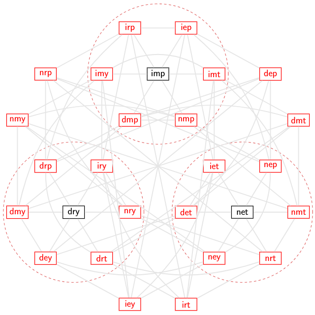
The valid words are shown in black; the invalid words are shown in red. The thin gray lines, which make this graph look like one of the back pages in an airline magazine that shows all the routes between cities, show adjacency where only one symbol change is required. The dashed red circles enclose both the valid words and all invalid words that are immediately adjacent to a valid word. Here we can correct one error by noting that the words within the circles have only one nearest valid word; as we said before, receiving drt probably means that it was originally dry. Some messages are not immediately adjacent to a valid word, like nmy, so they lie outside the red circles, and there is no unambiguous “nearest” valid word.
This is a fairly simple encoding scheme; it lets us correct up to one error, and detect up to two errors (three errors can get us from one valid word to another valid word), at the cost of 3 symbols per word.
Okay, here we have to stop and define some important terms that are commonly used in the subject of communications and coding theory:
- bit — the smallest possible unit of information, either a 0 or 1.
- symbol — a unit of information used in a particular type of code. For example, bytes (8-bit values) are one way of expressing a symbol. The set of all symbols in a particular code is finite, but could be as small as a bit, and arbitrarily large. In practical systems, they are often elements of some finite field \( GF(2^N) \) for some value of \( N \).
- block code — this type of encoding takes a fixed number of input symbols (the input block), and converts them to a fixed number of output symbols (the output block) in a functional manner — in other words, identical input blocks yield the same output block. Block codes typically are parameterized in terms of \( (n,k) \) where \( n \) is the number of output symbols and \( k \) is the number of input symbols. For example, a \( (255, 239) \) Reed-Solomon code with eight-bit symbols takes a block of 239 input bytes and encodes them as a block of 255 output bytes, adding 16 bytes of redundancy.
- codeword — a valid output block from a block code is called a codeword.
-
Hamming distance — the number of symbol changes required to get from one possible block to another block, on an adjacency graph of the possible blocks expressible in a code.
-
minimum Hamming distance — the minimum Hamming distance of any code is the minimum Hamming distance between any two distinct codewords. This is usually denoted \( d \) (or sometimes \( d^* \)), and there are theorems that state for a code with minimum distance \( d \), up to \( d-1 \) errors can be detected, and up to \( \lfloor\frac{d-1}{2}\rfloor \) errors can be corrected — although not at the same time, as we’ll note later. In the
dry imp netcode, the minimum Hamming distance is 3; up to 2 errors can be detected and 1 error can be corrected. With a \( (255,239) \) Reed-Solomon code, the minimum Hamming distance is \( n-k+1 = 17 \), and the code can correct up to \( t=\lfloor\frac{17-1}{2}\rfloor = 8 \) errors, and detect up to \( 2t=16 \) errors. - linear code — these are codes where any linear combination of codewords creates another valid codeword. Codes based around finite fields tend to be linear, and they have some properties that simplify analysis.
- code rate — this is the space efficiency of a code; for an \( (n,k) \) block code, the code rate is \( k/n \). A \( (255,239) \) Reed-Solomon code has code rate of about 0.9373. The
dry imp netcode has a code rate of 1/3.
The dry imp net code is a practical code. But it has a lot of “three-ness” which keeps it from being a good match to something computerized. Computers use binary, so practical examples of error-detecting codes and error-correcting codes usually have some power of two of symbols — the symbols are either bits, or groups of bits. Let’s look at one of these.
Simple Examples: Parity and Checksums
The easiest way to add some redundancy in a binary-based system is a modulo calculation.
I could, for example, calculate a parity bit. Let’s say that I had the ASCII character E, represented as hex 0x45 or binary 01000101. If I take all eight bits and XOR them together, I’ll get a 1, and I can concatenate the resulting parity bit with the input bits to create a nine-bit encoded symbol 010001011. This encoding has a minimum Hamming distance of 2, and provides enough information to detect one bit error, whether it occurs in the eight data bits or in the parity bit. It is not possible to detect more than one error, and it is not possible to correct any error, at least not with parity encoding alone.
Or I could calculate a bytewise checksum, taking the sum of bytes:
def checksum(msg):
    return sum(ord(b) for b in msg) & 0xff

def print_checksum(msg):
    print "%02x %s" % (checksum(msg), msg)

print_checksum("Ernie, you have a banana in your ear!")
print_checksum("Ernie, you h<ve a banana in your ear!")
c1 Ernie, you have a banana in your ear! 9c Ernie, you h<ve a banana in your ear!
I could either concatenate the checksum, or the negative of the checksum, to the end of the message. The negative of the checksum is useful in some ways. Let’s say \( C(x) \) is the checksum function. Then \( C(M \mid -C(M)) = 0 \) — that is, if I take the original text and concatenate the negative of the checksum, and use that as the transmitted message, and put it through the checksum function, I will get zero as a result. If I receive a message and calculate a nonzero checksum, then something is wrong.
This helps; it’s better than nothing, but it’s not that great. You might think that this would be able to detect several errors, but its minimum Hamming distance is still 2, meaning it can only guarantee detection of one byte error (since the symbols here are bytes, not bits) and cannot correct any errors. Unfortunately, errors in the same bit of two different bytes will cancel out changes in the checksum:
print_checksum("Ernie, you have a banana in your ear!")
print_checksum("Ernie, you have a abnana in your ear!")
c1 Ernie, you have a banana in your ear! c1 Ernie, you have a abnana in your ear!
Still, I mention a checksum here, in part because I benefited from it personally. From about 1984 to 1990 I did all my school reports on a Commodore 64 running SpeedScript, a limited but reasonably functional word processor for editing ASCII text, published by Compute’s Gazette in 1984. SpeedScript was a binary executable for 6502 and 6510 processors, and since the standard practice of both Compute! and Compute’s Gazette was for subscribers to produce working programs on their computers by typing in program listings, there had to be a way to type in the contents of that binary executable. I had typed in a BASIC program called MLX, which let you type in a series of byte values, as integers, and it would enter them into the computer’s memory, one byte at a time. (255 252 208 254 192 65 ...) The original version of MLX used listings of six data bytes and one checksum byte per line, so that if there was a single byte error, the program would catch it and prompt you to retype the line. Somehow I convinced my mother to type in the listing for SpeedScript for me, and we saved it on disk, using it on many occasions over the next 6 years. Because it used simple checksums, this version of MLX could not detect two transposed bytes, but a later version of MLX used a more sophisticated hashing algorithm.
The rest of this article touches upon some more useful linear codes; what they have in common with parity and checksums is that the redundancy in the messages comes from a remainder calculation. Instead of integer division, however, the remainder is computed in a finite field, and because of the nifty properties of finite fields, we get some superior error-detecting and error-correcting abilities that are better than what we can get out of a parity bit or simple checksums. This division-in-finite-fields aspect also leads to the possible use of LFSRs for encoding and (in some cases) decoding.
Cyclic Redundancy Check (CRC)
Probably the most common error-detecting code used nowadays is the cyclic redundancy check or CRC. I’ve written about them before in an earlier article, but, at the time, I managed to sidestep the theory behind them. So we’re going to come back to it.
Perhaps you were wondering where the linear feedback shift registers come in. Well, here we are.
CRCs are based around a couple of parameters, things like bit order and initialization value, but the most important parameter to specify is a polynomial. This polynomial is the generating polynomial \( p(x) \), and is the same kind of \( p(x) \) we’ve been using in our discussions of quotient rings \( GF(2)[x]/p(x) \). Essentially, each coefficient of the polynomial represents a feedback term in a corresponding LFSR.
Way back in Part I I showed this diagram of a Galois-representation LFSR:
So far, all of the LFSRs we have used are autonomous: they have no external input; the LFSR state keeps updating, and as long as it’s a maximal-length LFSR, it cycles through all possible nonzero states. A hardware circuit to calculate CRCs uses an LFSR with external inputs from the bits of the data stream:
The input word in a CRC represents a polynomial. How? Well, for example, suppose we have an input message Hi! which is 48 69 21 in hexadecimal or 01001000 01101001 00100001 in binary. Each bit represents a different polynomial coefficient, so we can find the 1 bits and use them to designate the nonzero terms of the polynomial, or \( m(x) = x^{22} + x^{19} + x^{14} + x^{13} + x^{11} + x^8 + x^5 + 1. \)
for k in 'Hi!':
    print '{0:02x} {0:08b}'.format(ord(k))
48 01001000 69 01101001 21 00100001
Suppose our polynomial \( p(x) = x^{16} + x^{12} + x^3 + x + 1 \). We could find \( r(x) = x^{16} m(x) \bmod p(x) \):
from libgf2.gf2 import GF2QuotientRing, GF2Polynomial

m = GF2Polynomial(0x486921)
p = GF2Polynomial(0x1100b)

def describepoly(p):
    onebits = []
    c = p.coeffs
    i = 0
    while c > 0:
        if (c & 1) > 0:
            onebits.append(i)
        i += 1
        c >>= 1
    return list(reversed(onebits))

m_shift16 = GF2Polynomial(m.coeffs << 16)
r = m_shift16 % p

for item,name in ((m,"m"), (p,"p"), (r,"r")):
    print "%s=%06x %s" % (name, item.coeffs, describepoly(item))
m=486921 [22, 19, 14, 13, 11, 8, 5, 0]
p=01100b [16, 12, 3, 1, 0]
r=007ed3 [14, 13, 12, 11, 10, 9, 7, 6, 4, 1, 0]
This computation tells us that \( r(x) = x^{14} + x^{13} + x^{12} + x^{11} + x^{10} + x^9 + x^7 + x^6 + x^4 + x + 1 \), represented in hexadecimal as 7ed3.
Why \( r(x) = x^{16}m(x) \bmod p(x) \), rather than just \( r(x) = m(x) \bmod p(x) \)? And why \( x^{16} \) rather than, say, \( x^{13} \)? It’s because we’re calculating a 16-bit CRC, and we’ll see why in just a minute.
We could get the same result by shifting in bits one at a time; rather than computing a polynomial divide and remainder all at once, we incrementally compute some remainder \( r_k(x) = (xr_{k-1}(x) + x^{16}b_k) \bmod p(x) \) with \( b_k \) being the \( k \)th bit of the message, and \( r_{-1}(x) = 0 \). This effectively comes up with the same answer, and the LFSR update step does this computation. Since \( p(x) = x^{16} + x^{12} + x^3 + x + 1 \), this means that \( x^{16} \equiv x^{12} + x^3 + x + 1 \pmod{p(x)} \) and we can transform the computation to \( r_k(x) = (xr_{k-1}(x) + (x^{12} + x^3 + x + 1) b_k) \bmod p(x) \) — essentially XORing the “tail” of the polynomial 0x100b any time the bit \( b_k = 1 \).
def crc_bitwise(message, polynomial, init=0, final=0, lsb_first=True, verbose=False):
    field = GF2QuotientRing(polynomial)
    n = field.degree
    polytail = polynomial ^ (1<<n)
    # all bits of the polynomial except the leading one
    crc = init
    for byte in message:
        bytecode = ord(byte)
        if verbose:
            print "%s (0x%02x)" % (repr(byte), bytecode)
        for bitnum in xrange(8):
            i = bitnum if lsb_first else (7-bitnum)
            bit = (bytecode >> i) & 1
            crc_prev = crc
            crc_prev_double = field.mulraw(2,crc)
            crc = crc_prev_double ^ (polytail if bit else 0)
            if verbose:
                print "%d %04x -> %04x -> %04x" % (bit, crc_prev, crc_prev_double, crc)
    if final:
        if verbose:
            print "%04x ^ %04x = %04x" % (crc, final, crc^final)
        crc ^= final
    # bit reverse within bytes
    if lsb_first:
        out = 0
        for k in xrange(n):
            out <<= 1
            out ^= (crc >> ((n-1-k)^7)) & 1
        if verbose:
            print "reversed(%04x) = %04x" % (crc, out)
        crc = out
    return crc

'%04x' % crc_bitwise('Hi!', 0x1100b, lsb_first=False, verbose=True)
'H' (0x48) 0 0000 -> 0000 -> 0000 1 0000 -> 0000 -> 100b 0 100b -> 2016 -> 2016 0 2016 -> 402c -> 402c 1 402c -> 8058 -> 9053 0 9053 -> 30ad -> 30ad 0 30ad -> 615a -> 615a 0 615a -> c2b4 -> c2b4 'i' (0x69) 0 c2b4 -> 9563 -> 9563 1 9563 -> 3acd -> 2ac6 1 2ac6 -> 558c -> 4587 0 4587 -> 8b0e -> 8b0e 1 8b0e -> 0617 -> 161c 0 161c -> 2c38 -> 2c38 0 2c38 -> 5870 -> 5870 1 5870 -> b0e0 -> a0eb '!' (0x21) 0 a0eb -> 51dd -> 51dd 0 51dd -> a3ba -> a3ba 1 a3ba -> 577f -> 4774 0 4774 -> 8ee8 -> 8ee8 0 8ee8 -> 0ddb -> 0ddb 0 0ddb -> 1bb6 -> 1bb6 0 1bb6 -> 376c -> 376c 1 376c -> 6ed8 -> 7ed3
'7ed3'
More practical software implementations of CRCs use table lookups to handle CRC updates one byte at a time, rather than one bit at a time. But a hardware implementation can be really simple if it just implements the appropriate LFSR, with input bits coming one at a time from the message.
Also, most CRCs use an initial and a final value. The final value is just a value that is XORd in at the end. The initial value is usually all ones (0xFFFF for a 16-bit CRC), so that if the message starts with any zero bytes, changing the number of zero bytes changes the CRC. If the initial value is 0, then the CRC doesn’t change if we add a zero byte:
'%04x' % crc_bitwise('\x00\x00Hi!', 0x1100b, lsb_first=False, verbose=True)'\x00' (0x00) 0 0000 -> 0000 -> 0000 0 0000 -> 0000 -> 0000 0 0000 -> 0000 -> 0000 0 0000 -> 0000 -> 0000 0 0000 -> 0000 -> 0000 0 0000 -> 0000 -> 0000 0 0000 -> 0000 -> 0000 0 0000 -> 0000 -> 0000 '\x00' (0x00) 0 0000 -> 0000 -> 0000 0 0000 -> 0000 -> 0000 0 0000 -> 0000 -> 0000 0 0000 -> 0000 -> 0000 0 0000 -> 0000 -> 0000 0 0000 -> 0000 -> 0000 0 0000 -> 0000 -> 0000 0 0000 -> 0000 -> 0000 'H' (0x48) 0 0000 -> 0000 -> 0000 1 0000 -> 0000 -> 100b 0 100b -> 2016 -> 2016 0 2016 -> 402c -> 402c 1 402c -> 8058 -> 9053 0 9053 -> 30ad -> 30ad 0 30ad -> 615a -> 615a 0 615a -> c2b4 -> c2b4 'i' (0x69) 0 c2b4 -> 9563 -> 9563 1 9563 -> 3acd -> 2ac6 1 2ac6 -> 558c -> 4587 0 4587 -> 8b0e -> 8b0e 1 8b0e -> 0617 -> 161c 0 161c -> 2c38 -> 2c38 0 2c38 -> 5870 -> 5870 1 5870 -> b0e0 -> a0eb '!' (0x21) 0 a0eb -> 51dd -> 51dd 0 51dd -> a3ba -> a3ba 1 a3ba -> 577f -> 4774 0 4774 -> 8ee8 -> 8ee8 0 8ee8 -> 0ddb -> 0ddb 0 0ddb -> 1bb6 -> 1bb6 0 1bb6 -> 376c -> 376c 1 376c -> 6ed8 -> 7ed3
'7ed3'
Now here’s where that \( x^{16} \) comes in. One important aspect of any CRC is that if you compute the CRC of a message appended with the message’s CRC, the result should be constant. With no initialization value or final value, that constant is zero.
Mathematically, we’re computing \( r(x) = x^{16}m(x) \bmod p(x) \), so if we let \( m’(x) = x^{16}m(x) + r(x) \) (essentially concatenating \( r(x) \) to the end of the message) then \( m’(x) \bmod p(x) = 0 \) and that means that the remainder \( r’(x) = x^{16}m’(x) \bmod p(x) = 0 \).
For example:
def crc1(message):
    return crc_bitwise(message, 0x1100b, lsb_first=False)

def crc2(message):
    return crc_bitwise(message, 0x11021, lsb_first=True, init=0xffff, final=0xffff)

for crcfunc in crc1, crc2:
    print ""
    print crcfunc.__name__
    for message in ["Hi!","squirrels","Ernie, you have a banana in your ear!"]:
        print message
        crc =  crcfunc(message)
        crc2 = crcfunc(message+chr(crc>>8)+chr(crc&0xff))
        print "crc(message) = %04x; crc(message|crc(message)) = %04x" % (crc, crc2);
crc1 Hi! crc(message) = 7ed3; crc(message|crc(message)) = 0000 squirrels crc(message) = 2eef; crc(message|crc(message)) = 0000 Ernie, you have a banana in your ear! crc(message) = 2fed; crc(message|crc(message)) = 0000 crc2 Hi! crc(message) = be84; crc(message|crc(message)) = 470f squirrels crc(message) = 9412; crc(message|crc(message)) = 470f Ernie, you have a banana in your ear! crc(message) = 3fc0; crc(message|crc(message)) = 470f
The reason this is important is that the message and its appended CRC comprises a codeword \( c(x) \) which has constant remainder modulo \( p(x) \); this gives the codeword certain advantageous properties, and makes it fairly straightforward to analyze for things like Hamming distance. For example, suppose we had two \( n \)-bit codewords. What’s the minimum Hamming distance? In this case, since \( c_1(x) = q_1(x)p(x) + r(x) \) and \( c_2(x) = q_2(x)p(x) + r(x) \), it means that \( p(x) \) divides \( e(x) = c_1(x) - c_2(x) \) and we are looking for a polynomial \( e(x) \) that has a minimum number of nonzero terms and is a multiple of \( p(x) \).
Let’s take the polynomial \( p_8(x) = x^8 + x^4 + x^3 + x^2 + 1 \) (0x11D), for example. Like all primitive polynomials, this divides \( x^{2^8 - 1} + 1 = x^{255} + 1 \), which has two nonzero terms, so 256-bit encoded messsages (31 bytes data + 1-byte CRC) have a minimum Hamming distance of 2. What about a Hamming distance of 3?
from libgf2.gf2 import _GF2

p8 = 0x11D
def hunt_for_trinomial_multiple_slow(p, max_degree=128):
    for c1 in xrange(2, max_degree):
        for c2 in xrange(1, c1):
            if _GF2.mod(1 + (1<<c1) + (1<<c2), p) == 0:
                return (1, c2, c1)

def hunt_for_trinomial_multiple(p, max_degree=128):
    """
    Find trinomials that are a multiple of p.
    This is optimized.
    """
    r = _GF2.mod(2,p)
    remainder_list = [1, r]
    remainder_map = {1: 0, r: 1}
    for c1 in xrange(2,max_degree):
        # r = x^c1 mod p
        r = _GF2.mod(r<<1, p)
        remainder_list.append(r)
        remainder_map[r] = c1
        # look for some r2 = x^c2 mod p, such that 1 + r + r2 = 0
        c2 = remainder_map.get(1^r)
        if c2 is not None and (c2 != 0):
            return (1, c2, c1)
hunt_for_trinomial_multiple(p8)
(1, 10, 21)
It turns out that \( e(x) = x^{21} + x^{10} + 1 \) is a multiple of \( p_8(x) = x^8 + x^4 + x^3 + x^2 + 1 \), so this forms an error pattern flipping three bits of the message to leave the same CRC.
def hexlify(message):
    return ' '.join('%02x' % ord(c) for c in message)
for message in ['Hi!', 'Hi!\x7f', 'HI%\x7e', 'Neato', 'Neato\x72', 'NeaTk\x73']:
    print "message = %s (%s)"  % (repr(message), hexlify(message))
    print "crc = %02x" % crc_bitwise(message, 0x11D, lsb_first=False)
message = 'Hi!' (48 69 21) crc = 7f message = 'Hi!\x7f' (48 69 21 7f) crc = 00 message = 'HI%~' (48 49 25 7e) crc = 00 message = 'Neato' (4e 65 61 74 6f) crc = 72 message = 'Neator' (4e 65 61 74 6f 72) crc = 00 message = 'NeaTks' (4e 65 61 54 6b 73) crc = 00
Here I flipped bits 0 (bit 0 of the last byte), bit 10 (bit 2 of the 2nd-to-last byte), and bit 21 (bit 5 of the 3rd-to-last byte) of the encoded message, and I get the same result — showing by example that we can show valid codewords three bit flips apart, with these bits being in three neighboring bytes.
With 16-bit CRCs, the situation is quite a bit better. All primitive degree-16 polynomials divide \( x^{65535} + 1 \), so the only way to “fool” a 16-bit CRC with two bit errors that leave the CRC unchanged, is to have a message with at least 65536 bits (8192 bytes). As far as three-bit errors that leave the CRC unchanged — it varies by the polynomial \( p(x) \), but the smallest trinomial multiple may have a degree in the hundreds. The 16-bit primitive polynomial champions are 11b2b and 1a9b1 which have a trinomial multiple that is a degree of 1165. Some polynomials which are not primitive have no trinomial multiples — if \( p(1) = 0 \) then there are no trinomial multiples. (The X.25 CRC polynomial is \( x^{16} + x^{12} + x^5 + 1 \), which is not a primitive polynomial.)
from libgf2.gf2 import checkPeriod

nprim = 0
for p in xrange(65537,131072,2):
    # Find all primitive 16-bit polynomials
    if checkPeriod(p,65535) == 65535:
        nprim += 1
        tri = hunt_for_trinomial_multiple(p, max_degree=2000)
        if nprim < 20 or tri[2] > 900:
            print '%5x -> %s' % (p,tri)
1002d -> (1, 543, 567) 10039 -> (1, 245, 408) 1003f -> (1, 67, 360) 10053 -> (1, 97, 247) 100bd -> (1, 350, 353) 100d7 -> (1, 49, 332) 1012f -> (1, 19, 198) 1013d -> (1, 35, 432) 1014f -> (1, 203, 242) 1015d -> (1, 149, 314) 10197 -> (1, 185, 251) 101a1 -> (1, 55, 239) 101ad -> (1, 40, 221) 101bf -> (1, 29, 215) 101c7 -> (1, 131, 153) 10215 -> (1, 75, 391) 10219 -> (1, 84, 215) 10225 -> (1, 423, 439) 1022f -> (1, 684, 725) 11753 -> (1, 626, 1161) 11ae3 -> (1, 245, 998) 11b2b -> (1, 544, 1165) 1370b -> (1, 916, 1019) 13c6f -> (1, 814, 915) 13d07 -> (1, 99, 1078) 13d83 -> (1, 611, 935) 14495 -> (1, 117, 1051) 15245 -> (1, 934, 1051) 16143 -> (1, 213, 964) 1650f -> (1, 663, 1014) 1725f -> (1, 107, 910) 1828b -> (1, 133, 983) 18379 -> (1, 324, 935) 184cf -> (1, 325, 957) 1850d -> (1, 751, 964) 18eb1 -> (1, 753, 998) 195d1 -> (1, 535, 1161) 19a6f -> (1, 872, 971) 19bef -> (1, 764, 997) 1a1d9 -> (1, 103, 1019) 1a283 -> (1, 850, 983) 1a9b1 -> (1, 621, 1165) 1b0ef -> (1, 595, 1019) 1c179 -> (1, 979, 1078) 1e14d -> (1, 351, 1014) 1e643 -> (1, 632, 957) 1ec79 -> (1, 101, 915) 1ecb3 -> (1, 99, 971) 1ee1b -> (1, 424, 1019) 1efb3 -> (1, 233, 997) 1f49d -> (1, 803, 910)
The point is that the difference between an 8-bit, a 16-bit, and a 32-bit CRC isn’t just that the odds of a CRC collision of two arbitrary messages are \( 1/256 \), \( 1/65536 \), and \( 1/4294967296 \). It’s that if errors are relatively uncommon and bounded — that is, we suspect there is some value \( B \) such that the number of errors is always less than or equal to \( B \) — there may be short messages for which we can guarantee we will be able to detect errors, because the Hamming distance between any two messages of this length is greater than \( B \). As the messages get longer, then there are more opportunities for a small number of errors to be undetectable with a given type of CRC. These errors have to be in just the right places, so it’s not a very likely scenario, but it’s possible.
Philip Koopman at Carnegie-Mellon maintains the “CRC Zoo” which lists known Hamming distances for various polynomials. For example, the 16-bit polynomial represented by 11b2b = \( x^{16} + x^{12} + x^{11} + x^9 + x^8 + x^5 + x^3 + x + 1 \) has these properties:
- 65535 bits (65519 data bits) is the maximum number of bits with Hamming distance = 3
- 1165 bits (1149 data bits) for HD=4
- 78 bits (62 data bits) for HD=5
- 35 bits (19 data bits) for HD=6
A 32-bit CRC improves error detection significantly; the Ethernet CRC — used also in PNG — basically protects all valid Ethernet frames (up to roughly 1500 bytes = 12000 bits) against any 3 errors by having a minimum Hamming distance of 4. (Interestingly, Koopman has found other 32-bit polynomials with better Hamming distance properties.)
Error Correction: Hamming Codes
Hamming codes were invented in 1950 by Richard Hamming, and are a way of adding parity bits to form a code with minimum distance of 3. Because the symbols in Hamming codes are individual bits, they are very simple to understand and to implement. I love the history behind Hamming’s discovery as noted in Wikipedia; it truly is one of those necessity-is-the-mother-of-invention stories:
Richard Hamming, the inventor of Hamming codes, worked at Bell Labs in the 1940s on the Bell Model V computer, an electromechanical relay-based machine with cycle times in seconds. Input was fed in on punched paper tape, seven-eighths of an inch wide which had up to six holes per row. During weekdays, when errors in the relays were detected, the machine would stop and flash lights so that the operators could correct the problem. During after-hours periods and on weekends, when there were no operators, the machine simply moved on to the next job.
Hamming worked on weekends, and grew increasingly frustrated with having to restart his programs from scratch due to detected errors. In a taped interview Hamming said, “And so I said, ‘Damn it, if the machine can detect an error, why can’t it locate the position of the error and correct it?’” [3] Over the next few years, he worked on the problem of error-correction, developing an increasingly powerful array of algorithms. In 1950, he published what is now known as Hamming Code, which remains in use today in applications such as ECC memory.
Anyway, the usual example is the (7,4) Hamming code, which has 4 data bits and 3 parity bits. Here is one possible matrix that helps define this code:
$$ \begin{bmatrix}G\cr\hdashline H\end{bmatrix} = \left[ \begin{array}{c:c}G^T & H^T \end{array}\right] = \left[ \begin{array}{c:c} I & A^T \\ \hdashline A & I \\ \end{array}\right] = \left[\begin{array}{cccc:ccc} 1 & 0 & 0 & 0 & 1 & 1 & 0 \cr 0 & 1 & 0 & 0 & 0 & 1 & 1 \cr 0 & 0 & 1 & 0 & 1 & 1 & 1 \cr 0 & 0 & 0 & 1 & 1 & 0 & 1 \cr \hdashline 1 & 0 & 1 & 1 & 1 & 0 & 0 \cr 1 & 1 & 1 & 0 & 0 & 1 & 0 \cr 0 & 1 & 1 & 1 & 0 & 0 & 1 \cr \end{array}\right] $$
The upper rows, \( G \), are called the generator matrix, and these consist of an identity matrix (4x4 in this case) along with a special matrix \( A \) that can be used to compute parity bits.
If the data bits are \( D = \begin{bmatrix}d_0 & d_1 & d_2 & d_3\end{bmatrix} \), then the parity bits are computed as \( P = \begin{bmatrix}p_0 & p_1 & p_2\end{bmatrix} = DA^T \); the codeword is formed as \( C = \left[\begin{array}{c:c}D&DA^T\end{array}\right] = DG. \) For those of you who don’t like matrices, this can be written in scalar form as a series of equations:
$$\begin{align} p_0 &= a_{00}d_0 + a_{01}d_1 + a_{02}d_2 + a_{03}d_3 \cr p_1 &= a_{10}d_0 + a_{11}d_1 + a_{12}d_2 + a_{13}d_3 \cr p_2 &= a_{20}d_0 + a_{21}d_1 + a_{22}d_2 + a_{23}d_3 \end{align}$$
With the specific bit patterns in \( A \), this works out to be
$$\begin{align} p_0 &= d_0 + d_2 + d_3 \cr p_1 &= d_0 + d_1 + d_2 \cr p_2 &= d_1 + d_2 + d_3 \end{align}$$
so, for example, the data block \( d_0d_1d_2d_3 \) = 1011 would be encoded as 1011010, by appending three parity bits onto the end.
Decoding is similar; we use the lower rows \( H \), called the parity-check matrix, to compute a syndrome vector \( S =\left[\begin{array}{c:c}D&P\end{array}\right] H^T = CH^T \); for the matrix above, this translates to
$$\begin{align} s_0 &= d_0 + d_2 + d_3 + p_0 \cr s_1 &= d_0 + d_1 + d_2 + p_1 \cr s_2 &= d_1 + d_2 + d_3 + p_2 \end{align}$$
Note that this is the same calculation as the parity bit calculation, but with the received parity bit — which may be different then the transmitted parity bit — added. If there were no errors, the syndrome bits would be zero. If there is an error, we can use the syndrome bits to locate the error:
import pandas as pd

data = []
for error_pos in xrange(-1,7):
    codeword = [0]*7
    if error_pos == -1:
        syndrome = [0,0,0]
    else:
        codeword[error_pos] = 1
        syndrome = [codeword[0] ^ codeword[2] ^ codeword[3] ^ codeword[4],
                    codeword[0] ^ codeword[1] ^ codeword[2] ^ codeword[5],
                    codeword[1] ^ codeword[2] ^ codeword[3] ^ codeword[6]]
    data.append([error_pos+1]+codeword+syndrome)
df = pd.DataFrame(data, columns=['error_pos+1','d0','d1','d2','d3',
                                 'p0','p1','p2','s0','s1','s2'])
df| error_pos+1 | d0 | d1 | d2 | d3 | p0 | p1 | p2 | s0 | s1 | s2 | |
|---|---|---|---|---|---|---|---|---|---|---|---|
| 0 | 0 | 0 | 0 | 0 | 0 | 0 | 0 | 0 | 0 | 0 | 0 |
| 1 | 1 | 1 | 0 | 0 | 0 | 0 | 0 | 0 | 1 | 1 | 0 |
| 2 | 2 | 0 | 1 | 0 | 0 | 0 | 0 | 0 | 0 | 1 | 1 |
| 3 | 3 | 0 | 0 | 1 | 0 | 0 | 0 | 0 | 1 | 1 | 1 |
| 4 | 4 | 0 | 0 | 0 | 1 | 0 | 0 | 0 | 1 | 0 | 1 |
| 5 | 5 | 0 | 0 | 0 | 0 | 1 | 0 | 0 | 1 | 0 | 0 |
| 6 | 6 | 0 | 0 | 0 | 0 | 0 | 1 | 0 | 0 | 1 | 0 |
| 7 | 7 | 0 | 0 | 0 | 0 | 0 | 0 | 1 | 0 | 0 | 1 |
Here we have a table showing all single-bit error possibilities in a codeword of all zeros. The data bits \( d_0d_1d_2d_3 \) are shown, along with parity bits \( p_0p_1p_2 \), and syndrome bits \( s_0s_1s_2 \). It is fairly easy to show that if there is at most one error, then either the syndrome bits are either all zeros, if no errors occur, or \( s(x) = s_2x^2 + s_1x + s_0 = x^j \alpha \bmod p(x) \) for \( p(x) = x^3 + x + 1 \) and \( \alpha = x + 1 \) with \( j \) being the error position, if one error occurs. The values \( p(x) \) and \( \alpha \) are different for each possible Hamming code, but if we know \( p(x) \) and \( \alpha \) we can create the appropriate generator and parity check matrices.
What this effectively means is that we can take the syndrome bits, calculate a discrete logarithm and it will tell us where the error is.
import libgf2.gf2

f3 = libgf2.gf2.GF2QuotientRing(0b1011)
alpha = 3
for j in xrange(7):
    print 'j=%d s0s1s2 = %s' % (j, ''.join(reversed('{0:03b}'.format(f3.lshiftraw(alpha,j)))))
j=0 s0s1s2 = 110 j=1 s0s1s2 = 011 j=2 s0s1s2 = 111 j=3 s0s1s2 = 101 j=4 s0s1s2 = 100 j=5 s0s1s2 = 010 j=6 s0s1s2 = 001
Hamming’s original (7,4) code had a clever transposition of bits that allowed the syndrome bits to be used directly to indicate where the error was, without requiring any discrete logarithm. But this required the parity bits and data bits to be interleaved, making a non-systematic code. Those of us who are a little obsessive-compulsive really like systematic codes, where the parity bits just get concatenated onto the end of the data bits, and everything stays together in its own group, nice and neat. After all, wouldn’t you rather see \( \begin{array}{c:c}d_0d_1d_2d_3&p_0p_1p_2\end{array} \) than \( p_0p_1d_0p_2d_1d_2d_3 \)? I know I would.
Hamming Codes with LFSRs
We can do the same kinds of calculations in hardware, using an LFSR, for both encoding and decoding Hamming code; for example suppose I had the code above with \( p(x) = x^3 + x + 1 \) and \( \alpha = x+1 = x^3 \bmod p(x) \), and data bits \( d_0d_1d_2d_3 = 1011 \). Calculating manually, we have
$$\begin{align} p_0 &= d_0 + d_2 + d_3 = 1 + 1 + 1 = 1\cr p_1 &= d_0 + d_1 + d_2 = 1 + 0 + 1 = 0\cr p_2 &= d_1 + d_2 + d_3 = 0 + 1 + 1 = 0 \end{align}$$
and this means our codeword is (in least-significant bit first) 1011100, or (in most-significant bit first) \( p_2p_1p_0d_3d_2d_1d_0 = \)0011101. We can get the same parity bits 001 by taking the value \( d_3d_2d_1d_0 \) and clocking it into an LFSR with some additional zero bits to take care of \( \alpha = x^3 \).
Similarly if we have \( d_3d_2d_1d_0 = \) 0010 then \( p_0 = 0, p_1 = 1, p_2 = 1 \) and our code word in most-signicant bit order is \( p_2p_1p_0d_3d_2d_1d_0 = \) 1100010.
def hamming74_encode(data):
    qr = GF2QuotientRing(0b1011)
    parity = 0
    bitpos = 1 << 3
    # clock in bit 3, then bit 2, then bit 1, then bit 0, then three zero bits
    for k in xrange(7):
        parity = qr.lshiftraw1(parity)
        if data & bitpos:
            parity ^= 1
        bitpos >>= 1
    return (parity << 4) | data

for data in [0b0000, 0b1101, 0b0010]:
    print "{0:04b} -> {1:07b}".format(data, hamming74_encode(data))
0000 -> 0000000 1101 -> 0011101 0010 -> 1100010
def hamming74_decode(codeword, return_syndrome=False):
    qr = GF2QuotientRing(0b1011)
    beta = 0b111
    syndrome = 0
    bitpos = 1 << 7
    # clock in the codeword, then three zero bits
    for k in xrange(10):
        syndrome = qr.lshiftraw1(syndrome)
        if codeword & bitpos:
            syndrome ^= 1
        bitpos >>= 1
    data = codeword & 0xf
    if syndrome == 0:
        error_pos=None
    else:
        # there are easier ways of computing a correction
        # to the data bits (I'm just not familiar with them)
        error_pos=qr.log(qr.mulraw(syndrome,beta))
        if error_pos < 4:
            data ^= (1<<error_pos)
    if return_syndrome:
        return data, syndrome, error_pos
    else:
        return data

for recv_word in [
    0b0000000,
    0b0000001,  # error in bit 0
    0b0000010,  # error in bit 1
    0b0000100,  # error in bit 2
    0b0001000,  # error in bit 3
    0b0010000,  # error in bit 4
    0b0100000,  # error in bit 5
    0b1000000,  # error in bit 6

    0b0011101,
    0b0011100,  # error in bit 0
    0b0011111,  # error in bit 1
    0b0011001,  # error in bit 2
    0b0010101,  # error in bit 3
    0b0001101,  # error in bit 4,
    0b0111101,  # error in bit 5,
    0b1011101,  # error in bit 6

    0b1100010,
    0b1100011,  # error in bit 0
    0b1100000,  # error in bit 1
    0b1100110,  # error in bit 2
    0b1101010,  # error in bit 3
    0b1110010,  # error in bit 4
    0b1000010,  # error in bit 5
    0b0100010,  # error in bit 6
    ]:
    data, syndrome, error_pos = hamming74_decode(recv_word, return_syndrome=True)
    print ("{0:07b} -> {1:04b} (syndrome={2:03b}, error_pos={3})"
           .format(recv_word, data, syndrome, error_pos))
0000000 -> 0000 (syndrome=000, error_pos=None) 0000001 -> 0000 (syndrome=100, error_pos=0) 0000010 -> 0000 (syndrome=011, error_pos=1) 0000100 -> 0000 (syndrome=110, error_pos=2) 0001000 -> 0000 (syndrome=111, error_pos=3) 0010000 -> 0000 (syndrome=101, error_pos=4) 0100000 -> 0000 (syndrome=001, error_pos=5) 1000000 -> 0000 (syndrome=010, error_pos=6) 0011101 -> 1101 (syndrome=000, error_pos=None) 0011100 -> 1101 (syndrome=100, error_pos=0) 0011111 -> 1101 (syndrome=011, error_pos=1) 0011001 -> 1101 (syndrome=110, error_pos=2) 0010101 -> 1101 (syndrome=111, error_pos=3) 0001101 -> 1101 (syndrome=101, error_pos=4) 0111101 -> 1101 (syndrome=001, error_pos=5) 1011101 -> 1101 (syndrome=010, error_pos=6) 1100010 -> 0010 (syndrome=000, error_pos=None) 1100011 -> 0010 (syndrome=100, error_pos=0) 1100000 -> 0010 (syndrome=011, error_pos=1) 1100110 -> 0010 (syndrome=110, error_pos=2) 1101010 -> 0010 (syndrome=111, error_pos=3) 1110010 -> 0010 (syndrome=101, error_pos=4) 1000010 -> 0010 (syndrome=001, error_pos=5) 0100010 -> 0010 (syndrome=010, error_pos=6)
Tada! Works like a charm.
Hamming codes are linear, which means that the sum of any two codewords is also a codeword (for example, 0011101 + 1100010 = 1111111), and the syndrome of the sum of any two received messages is equal to the sum of the syndrome of those two messages.
Something that will be useful later in our discussion of communications is to decode all possible patterns and look at how the decoder affects the number of errors. Since the Hamming code is linear, we can assume an intended message of 0000000 and see what the decoder does in each case.
# Find syndromes and error positions for basis vectors (all 1)
# and construct syndromes for all 128 possible values using linearity

syndrome_to_correction_mask = np.zeros(8, dtype=int)
patterns = np.arange(128)
syndromes = np.zeros(128, dtype=int)
bit_counts = np.zeros(128, dtype=int)
for i in xrange(7):
    error_pattern = 1<<i
    data, syndrome, error_pos = hamming74_decode(error_pattern, return_syndrome=True)
    assert error_pos == i
    syndrome_to_correction_mask[syndrome] = error_pattern
    bitmatch = (patterns & error_pattern) != 0
    syndromes[bitmatch] ^= syndrome
    bit_counts[bitmatch] += 1

correction_mask = syndrome_to_correction_mask[syndromes[patterns]]
corrected_patterns = patterns ^ correction_mask
received_error_count = bit_counts[corrected_patterns & 0xF]
# determine the number of errors in the corrected data bits

H74_table = pd.DataFrame(dict(pattern=patterns,
                       raw_error_count=bit_counts,
                       correction_mask=correction_mask,
                       corrected_pattern=corrected_patterns,
                       received_error_count=received_error_count
                       ),
                  columns=['pattern',
                        'correction_mask','corrected_pattern',
                        'raw_error_count','received_error_count'])
H74_table| pattern | correction_mask | corrected_pattern | raw_error_count | received_error_count | |
|---|---|---|---|---|---|
| 0 | 0 | 0 | 0 | 0 | 0 |
| 1 | 1 | 1 | 0 | 1 | 0 |
| 2 | 2 | 2 | 0 | 1 | 0 |
| 3 | 3 | 8 | 11 | 2 | 3 |
| 4 | 4 | 4 | 0 | 1 | 0 |
| 5 | 5 | 64 | 69 | 2 | 2 |
| 6 | 6 | 16 | 22 | 2 | 2 |
| 7 | 7 | 32 | 39 | 3 | 3 |
| 8 | 8 | 8 | 0 | 1 | 0 |
| 9 | 9 | 2 | 11 | 2 | 3 |
| 10 | 10 | 1 | 11 | 2 | 3 |
| 11 | 11 | 0 | 11 | 3 | 3 |
| 12 | 12 | 32 | 44 | 2 | 2 |
| 13 | 13 | 16 | 29 | 3 | 3 |
| 14 | 14 | 64 | 78 | 3 | 3 |
| 15 | 15 | 4 | 11 | 4 | 3 |
| 16 | 16 | 16 | 0 | 1 | 0 |
| 17 | 17 | 32 | 49 | 2 | 1 |
| 18 | 18 | 4 | 22 | 2 | 2 |
| 19 | 19 | 64 | 83 | 3 | 2 |
| 20 | 20 | 2 | 22 | 2 | 2 |
| 21 | 21 | 8 | 29 | 3 | 3 |
| 22 | 22 | 0 | 22 | 3 | 2 |
| 23 | 23 | 1 | 22 | 4 | 2 |
| 24 | 24 | 64 | 88 | 2 | 1 |
| 25 | 25 | 4 | 29 | 3 | 3 |
| 26 | 26 | 32 | 58 | 3 | 2 |
| 27 | 27 | 16 | 11 | 4 | 3 |
| 28 | 28 | 1 | 29 | 3 | 3 |
| 29 | 29 | 0 | 29 | 4 | 3 |
| ... | ... | ... | ... | ... | ... |
| 98 | 98 | 0 | 98 | 3 | 1 |
| 99 | 99 | 1 | 98 | 4 | 1 |
| 100 | 100 | 16 | 116 | 3 | 1 |
| 101 | 101 | 32 | 69 | 4 | 2 |
| 102 | 102 | 4 | 98 | 4 | 1 |
| 103 | 103 | 64 | 39 | 5 | 3 |
| 104 | 104 | 1 | 105 | 3 | 2 |
| 105 | 105 | 0 | 105 | 4 | 2 |
| 106 | 106 | 8 | 98 | 4 | 1 |
| 107 | 107 | 2 | 105 | 5 | 2 |
| 108 | 108 | 64 | 44 | 4 | 2 |
| 109 | 109 | 4 | 105 | 5 | 2 |
| 110 | 110 | 32 | 78 | 5 | 3 |
| 111 | 111 | 16 | 127 | 6 | 4 |
| 112 | 112 | 4 | 116 | 3 | 1 |
| 113 | 113 | 64 | 49 | 4 | 1 |
| 114 | 114 | 16 | 98 | 4 | 1 |
| 115 | 115 | 32 | 83 | 5 | 2 |
| 116 | 116 | 0 | 116 | 4 | 1 |
| 117 | 117 | 1 | 116 | 5 | 1 |
| 118 | 118 | 2 | 116 | 5 | 1 |
| 119 | 119 | 8 | 127 | 6 | 4 |
| 120 | 120 | 32 | 88 | 4 | 1 |
| 121 | 121 | 16 | 105 | 5 | 2 |
| 122 | 122 | 64 | 58 | 5 | 2 |
| 123 | 123 | 4 | 127 | 6 | 4 |
| 124 | 124 | 8 | 116 | 5 | 1 |
| 125 | 125 | 2 | 127 | 6 | 4 |
| 126 | 126 | 1 | 127 | 6 | 4 |
| 127 | 127 | 0 | 127 | 7 | 4 |
128 rows × 5 columns
Note how in most cases the number of received errors decreases, but in some cases, like 0000011 or 0001001 or 0001010, the two input errors are “corrected” to become three data errors. This making-errors-worse behavior is unavoidable if there are more errors than a particular code can correct.
Here’s a summary:
H74_stats = (H74_table
          .groupby(['raw_error_count','received_error_count'])
          .agg({'pattern': 'count'})
          .rename(columns={'pattern':'count'}))

H74_stats| count | ||
|---|---|---|
| raw_error_count | received_error_count | |
| 0 | 0 | 1 |
| 1 | 0 | 7 |
| 2 | 1 | 9 |
| 2 | 9 | |
| 3 | 3 | |
| 3 | 1 | 7 |
| 2 | 15 | |
| 3 | 13 | |
| 4 | 1 | 13 |
| 2 | 15 | |
| 3 | 7 | |
| 5 | 1 | 3 |
| 2 | 9 | |
| 3 | 9 | |
| 6 | 4 | 7 |
| 7 | 4 | 1 |
Hamming codes are possible to construct for any codeword length of \( 2^n-1 \) for \( n\geq 2 \); the data length supported is \( 2^n-1-n \): in other words, \( (3,1), (7,4), (15,11), (31,26), (63,57) \), etc.
Since they can correct only a single error, their applications are somewhat limited to situations where errors are rare, and the probability of two or more bit errors in a codeword is negligible. But that doesn’t mean Hamming codes aren’t widely used! You’ll find them in many implementations of error-correcting code (ECC) memory which is robust to single bit errors.
There’s one more important takeaway from this multiple-errors-making-things-worse behavior, which applies to any error correcting code, not just Hamming codes: if our receiver attempts to correct errors, we give up some of our ability to detect errors. Think back to dry imp net land, where there are 27 possible received messages. If we don’t try to correct errors, then any of the 24 invalid messages, like drt or iey, can be interpreted as a detected error; we can detect up to two errors in a message, no matter what the errors are. Three errors could transform dry to net and we would have no way to know whether there was an error. But we can detect two errors with 100% certainty. On the other hand, if we do try to correct errors, then a two-error message like dry being corrupted as ney will be decoded as net, which is the wrong correction, but we have no way of knowing that ney was actually dry with two errors; instead it looks like net with one error. So there’s a tradeoff: if you use error correction to try to reduce the error rate for cases where errors are infrequent (low noise), it may actually increase the error rate for cases where errors are more frequent (high noise).
Wrapup
Today we looked at some error correction and detection codes.
We saw how Bert and Ernie struggled with a noisy communication channel containing a banana. We looked briefly at the Shannon-Hartley equation for channel capacity, and looked at an example code — dry imp net — to understand some of the basic concepts of error detection and correction, like Hamming distance.
We covered simple parity bits and checksums, and saw how they did provide minimal help with error detection, but have serious weaknesses such as the inability to detect transposed symbols.
We looked at CRCs, which are very good at detecting a few bit errors, and Hamming codes, which are good at correcting one bit error. We saw how allowing error correction weakens the ability of error detection.
Next time we’re going to be looking at Reed-Solomon codes.
References
Books:
I don’t have any good book recommendations for error-correcting codes… but then again, the three ones that I have, I bought used for a total of \$17.31 on abebooks.com:
-
W. Wesley Peterson and E. J. Weldon, Jr., Error-Correcting Codes, MIT Press, 2nd edition, 1972. This is aimed at the mathematically adept computer scientist, with lots of abstract algebra and theorems. Peterson was one of the grand old men of error detection and correction; he’s responsible for the invention of the CRC, so I respect him — and how cool is it to be an engineering professor in Hawaii for 45 years? — but I don’t like this book.
-
Benjamin Arazi, A Commonsense Approach to the Theory of Error Correcting Codes, MIT Press, 1988. This sounded promising, and it is written much more informally than Peterson and Weldon, with a practical bent. There are lots of examples of circuits here. Sometimes, though, there are topics which are covered very thinly, or not at all, and although Arazi does show what is done in practice, it would be helpful to get a better understanding of why it works. The diagrams look like they were created on this brand new program at the time called Hypercard.
-
Richard E. Blahut, Theory and Practice of Error Control Codes, Addison-Wesley, 1983. (As I write this, I didn’t realize until just now that this was published by Addison-Wesley. I like Addison-Wesley. There are a lot of good technical books from Addison-Wesley, like Design Patterns, Programming Pearls and Knuth’s The Art of Computer Programming.) This book isn’t bad, kind of halfway between Peterson and Arazi. It does have lots of theorems and abstract algebra, but for the most part you’ll be able to get by if you can follow the math in Parts I-VI of this series, and it is a more practical book than Peterson and Weldon. There are about five chapters that are relevant to Reed-Solomon codes, so lots of meat here. Maybe one of these days when I give it another reread, I will finally understand how convolutional codes work.
Error-Correcting Codes:
- Gregory Mitchell, ARL-TR-4901: Investigation of Hamming, Reed-Solomon, and Turbo Forward Error Correcting Codes, US Army Research Laboratory, July 2009.
CRCs:
-
Justin Ray, Philip Koopman, Efficient High Hamming Distance CRCs for Embedded Networks, Dependable Systems and Networks conference, June 2006.
-
Philip Koopman, Kevin Driscoll, Brendan Hall, Selection of Cyclic Redundancy Code and Checksum Algorithms to Ensure Critical Data Integrity, Federal Aviation Administration Technical Report TC-14/49, March 2015.
© 2018 Jason M. Sachs, all rights reserved.
- Comments
- Write a Comment Select to add a comment
To post reply to a comment, click on the 'reply' button attached to each comment. To post a new comment (not a reply to a comment) check out the 'Write a Comment' tab at the top of the comments.
Please login (on the right) if you already have an account on this platform.
Otherwise, please use this form to register (free) an join one of the largest online community for Electrical/Embedded/DSP/FPGA/ML engineers:


