Chebyshev Approximation and How It Can Help You Save Money, Win Friends, and Influence People

Well... maybe that's a stretch. I don't think I can recommend anything to help you win friends. Not my forte.

But I am going to try to convince you why you should know about Chebyshev approximation, which is a technique for figuring out how you can come as close as possible to computing the result of a mathematical function, with a minimal amount of design effort and CPU power. Let's explore two use cases:

• Amy has a low-power 8-bit microcontroller and needs to compute \( \sqrt{x} \) (square root) to get an accurate estimate of RMS power dissipated in a current sense resistor. She's finding that the math library implementation for sqrt() takes a lot of CPU time, and she's short on free program memory space, and is wondering if there is another way to compute square roots that takes less time and program memory.
• Bill is designing a sulfur dioxide (SO₂) detector, with a sensor that outputs a voltage dependent on SO₂ gas concentration, and a microcontroller that converts that voltage to a reading of SO₂ concentration so it can be displayed. He's not greatly concerned about CPU time limitations, but somehow he has to figure out how to convert gas sensor voltage to a concentration, because the sensor is fairly nonlinear.

In Amy's case, she has a known function that seems difficult to compute. In Bill's case, he has an unknown function that he has to figure out how to model. These are both cases of function evaluation with two very different priorities. Both are on embedded systems, which brings me to the Central Hypothesis of Mathematical Computation on Embedded Systems (CHoMCoES? It needs a better name, and I don't feel like calling it the Sachs Hypothesis):

The only embedded systems that require precision floating-point computations are desktop calculators.

Let that sink in for a minute. Your computer is a wonderful thing. It can calculate pi to hundreds of decimal places in milliseconds, or model the airflow patterns around jet engine blades. The origins of the computer have been consistently centered around mathematical computation, with a huge surge of development around the end of the Second World War and through the early days of solid-state transistors. If you needed a computer in the 1940's and 1950's, it was for some precise mathematical calculation. Computers were very expensive to own and operate; if you needed a quick estimate of some math, there were slide rules. This was also the era where whole books were published containing tables of engineering functions, so that if you needed to calculate Bessel functions to 5 decimal places, you could do it by looking it up in a table.

The desktop computer uses a calculation strategy of "full machine precision": for a given bit representation, there is only one correct answer to sin(x), and it is the bit pattern that is the one yields the smallest error from the exact mathematical calculation. Someone has written and tested mathematical software libraries that do this, and from there on out, it's just a function call.

Embedded systems, on the other hand, tend to contain inexpensive processors that are doing things with analog-to-digital-converter measurements. You can do math to the full 53 bits of IEEE-754 double-precision, but if your ADC readings, or the signal conditioning that precedes them, are only accurate to 0.1% (10 bits), then mathematical errors will be dwarfed by the errors of signal conditioning.

When you have a system that can tolerate mathematical errors, and has computing resource limitations driven by cost, all of a sudden the priority of mathematical computing changes. Now we have to decide what we really need when we want to compute something.

Let's take Amy's problem first: we need to compute a square root.

That statement is only an overview of what is needed. There are two major decisions that need to be made up front:

• over what range of x does \( \sqrt{x} \) need to be computed?
• what kind of accuracy does \( \sqrt{x} \) need? (and how does it vary with x?)

General full-machine precision math libraries have easy answers to these questions: any input needs to be tolerated, and for each input there is one correct output, even if the correct output is an error (e.g. \( \sqrt{x} \) for negative inputs in systems that don't use complex numbers).

In the embedded system, the accuracy and range requirements are judgement calls.

Accuracy is an easy thing to understand: there are algorithms that take shortcuts to computing an expression, and the more inaccuracy can be tolerated, the more shortcuts can be taken.

The range requirement is a bit more subtle. Obviously you have to support the expected range of inputs to an algorithm, and maybe you want to leave some engineering margin. But why would it be more expensive to calculate \( \sqrt{x} \) over a larger range? If I were to tell you that I was much more concerned about the range of a computation than the accuracy, would you believe me?

Let's use a real example. Amy thinks she needs \( \sqrt{u} \) calculated over the range \( u \in [0.2, 5.0] \). Her first instinct is to go find her calculus textbook and look up Taylor Series:

How not to evaluate functions, part 1: Taylor Series

Here is the Taylor series for \( \sqrt{1+x} \):    (equation courtesy of Wikipedia)

But there's a little footnote saying this only works for x between -1 and 1, meaning it won't work to calculate \( \sqrt{2} \) or the square root of anything 2 or larger. For \( \sqrt{5} \), she has to use a trick, namely that \( \sqrt{5} \) = \( 2\times\sqrt{5/4} \). So she decides to limit the actual input range of the Taylor series to cover the range of \( \sqrt{1+x} \) for \( x \in [-0.8,+0.25] \), and if \( u = 1+x > 1.25 \) then Amy will do the divide-by-4 trick: (we'll use Python here; assume that Amy does something equivalent in C)

def sqrt1(x):
# returns sqrt(1+x) for x between -0.8 and +0.25
   return 1 + x/2 - x*x/8 + x*x*x/16
def sqrtapprox(u):
# valid for x between 0.2 to 5.0
   if (u >= 1.25):
      return sqrt1(u/4-1)*2
   else:
      return sqrt1(u-1)

Is this good enough? Hmm, let's think about this. We want to know the error between a function and its approximation(s). Let's graph that error. Here's a quick Python function that uses numpy and matplotlib to plot the results:

import numpy as np
import matplotlib.pyplot as plt
def showplots(f,approxlist,a,b):
    x = np.linspace(a,b,1000)
    plt.figure(1)
    plt.subplot(211)
    plt.plot(x,f(x))
    vfuncs = [np.vectorize(approx) for approx in approxlist]
    for vf in vfuncs:
        plt.plot(x,vf(x))
    plt.xlim(a,b)
    plt.ylabel('f(x) and approximations fa(x)')
    plt.subplot(212)
    for vf in vfuncs:
        plt.plot(x,f(x)-vf(x))
    plt.xlim(a,b)
    plt.ylabel('error = f(x)-fa(x)')
    plt.xlabel('x')
    plt.show()

The results of showplots(np.sqrt,[sqrtapprox],0.2,5.0) will show us the error between the full-machine-precision sqrt() and our approximation:

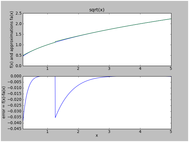
Yuck. A worst-case error of 0.038. Let's try some more terms in the Taylor series. That means we have to figure out how the coefficients work. A little pencil and paper algebra shows the coefficients starting from the quadratic term are $$\begin{eqnarray} a_2 &=& -\frac{1}{4\times 2} = -\frac{1}{8}, \cr a_3 &=& +\frac{3\times 1}{6\times 4\times 2} = \frac{1}{16}, \cr a_4 &=& -\frac{5\times 3\times 1}{8\times 6\times 4\times 2} = \frac{5}{128}, \cr a_5 &=& +\frac{7\times 5\times 3\times 1}{10\times 8\times 6\times 4\times 2} = \frac{7}{256}, \cr a_6 &=& -\frac{9\times 7\times 5\times 3\times 1}{12\times 10\times 8\times 6\times 4\times 2} = -\frac{21}{1024} \end{eqnarray}$$ and so on, so we try again:

def sqrt1a(x):
# returns sqrt(1+x) for x between -0.8 and +0.25
   return 1 + x/2 - x*x/8 + x*x*x/16 - 5.0/128*x*x*x*x
def sqrtapproxa(u):
# valid for x between 0.2 to 5.0
   if (u >= 1.25):
      return sqrt1a(u/4-1)*2
   else:
      return sqrt1a(u-1)
def sqrt1b(x):
# returns sqrt(1+x) for x between -0.8 and +0.25
   return 1 + x/2 - x*x/8 + x*x*x/16 - 5.0/128*x*x*x*x + 7.0/256*x*x*x*x*x
def sqrtapproxb(u):
# valid for x between 0.2 to 5.0
   if (u >= 1.25):
      return sqrt1b(u/4-1)*2
   else:
      return sqrt1b(u-1)

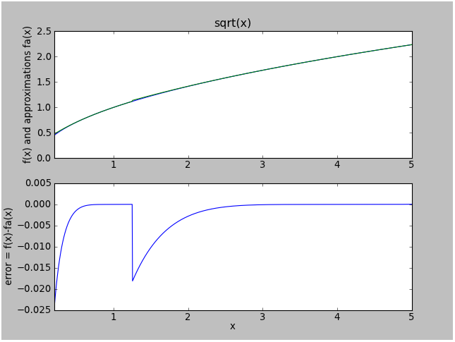
Here are the results for sqrtapproxa (a 4th-degree Taylor series):

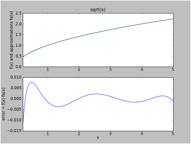
And here are the results for sqrtapproxb (a 5th-degree Taylor series):

Yuck. We added two more terms and we only got the error down to 0.015.

Here's what you need to learn about Taylor series for function evaluation. (Or rather, read this and whatever you don't understand, just trust me.)

To get the coefficients of a Taylor series for a function f in a region around a point \( x=x_0 \), you evaluate \( f(x_0) \) and all of the derivatives of \( f(x) \) at \( x=x_0 \). You don't have to look at the function anywhere else; the behavior at \( x=x_0 \) somehow lets you know what \( f(x) \) is elsewhere. For some functions (like \( \sqrt{1+x} \) ) the region of convergence is finite; for others like \( \sin x \) or \( e^x \) the region of convergence is everywhere.

Taylor series work on most everyday functions, because these functions have a property called "analyticity": all of their derivatives exist and are therefore continuous and smooth, and through the magic of mathematics this means that looking at an analytic function only at 1 point will tell you enough information to calculate it in some nearby region.

Right near \( x=x_0 \), Taylor series are great. The error between the exact function and the first N terms of the corresponding Taylor series will be extremely small around \( x=x_0 \). As you move away from \( x=x_0 \), the error starts to become larger. In general, the more terms you use, the better the approximation will be around \( x=x_0 \), but when the approximation starts to do poorly at the edge of its range, it diverges faster.

To sum this up: Taylor series approximations do not distribute the approximation error fairly. The error is small at \( x=x_0 \), but its error tends to be much larger at the edges of its range.

Now I'm going to show you two more attempts at approximating \( \sqrt{x} \) for \( x \in [0.2, 5.0] \), but I'm going to wait before explaining how I came up with them.

def sqrt1c(x):
# valid for x between 0.2 to 1.25
   coeffs = [0.20569678, -0.94612133, 1.79170646, -1.89014568, 1.66083189, 0.17814197]
   y = 0
   for c in coeffs:
      y = y * x + c
   return y
def sqrtapproxc(u):
# valid for u between 0.2 to 5.0
   if (u >= 1.25):
      return sqrt1c(u/4)*2
   else:
      return sqrt1c(u)
def sqrtapproxd(x):
# valid for x between 0.2 to 5.0
   coeffs = [0.00117581,-0.01915684,0.12329254,-0.41444219,1.04368339, 0.26700714]
   y = 0
   for c in coeffs:
      y = y * x + c
   return y

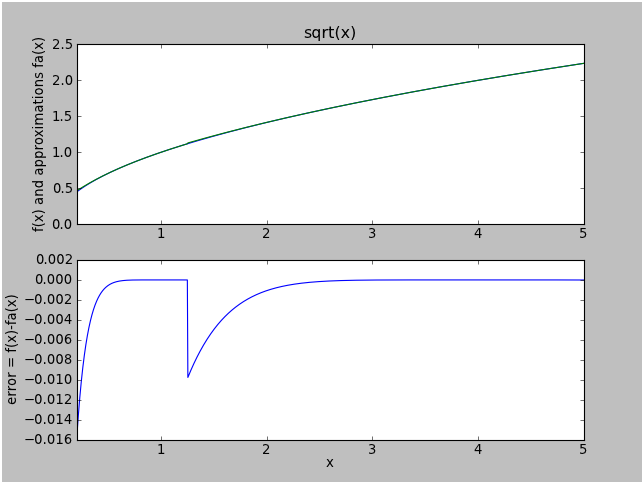
Approximation "c" splits the range between \( [0.2,1.25) \) and \( [1.25,5] \) as before; approximation "d" operates over the entire range \( [0.2,5] \). Both are 5th-degree polynomials. Here is the performance of approximation "c":

You'll notice a peak error of about 0.00042. This is about 35 times smaller than the error in approximation "b" (the Taylor series version using 5th order polynomials with the same range split).

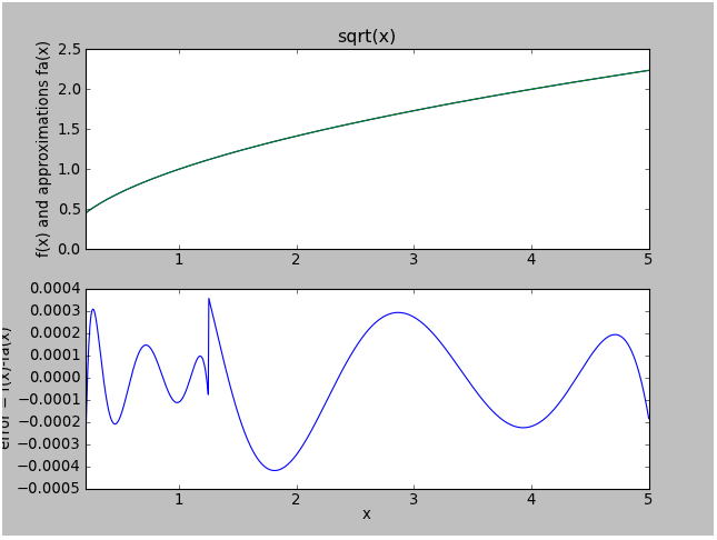
Here is the error for approximation "d":

That's about 0.011 worst case error, which is about 30% smaller than approximation "b". We got better worst-case error, without having to split up the range, with a polynomial of the same degree!

A few things to note from this exercise:

• Good function approximations have error graphs with a characteristic "wiggle". Ideally they form a so-called minimax function, where the positive and negative peaks all line up. This spreads the error throughout the range of input argument, and can be orders of magnitude better accuracy than a Taylor series polynomial of the same degree. In practice, it is difficult to achieve the ideal minimax error graph, but there is an easy method that comes close to it, which I'll explain in a bit.
• Range reduction can improve the accuracy of function evaluation significantly. Approximations "c" and "d" both used 5th degree polynomials, but approximation "d" used the whole input range (a 25:1 ratio of maximum to minimum input), whereas approximation "c" only used a part of the input range (with 6.25:1 ratio of maximum to minimum input), and "c" was 25 times more accurate.

How not to evaluate functions, part 2: lookup tables

All right, so let's toss out Taylor series. The next approach is a lookup table. The idea is simple: you have an array of precomputed values for your function, and use those as a table to evaluate the function. Let's look at a solution for \( \sqrt{x} \) over the \( [0.2, 5.0] \) range using a lookup table with 32 entries:

import math
def maketable0(func, a, b, n):
    table = func([(x+0.5)/n*(b-a)+a for x in range(0,n)])
    def tablefunc(x):
        if x < a or x > b:
            raise "out of range error"
        i = math.floor((x-a)/(b-a)*n)
        if i == n:
            i = n-1
        return table[i]
    return tablefunc
sqrtapproxe = maketable0(np.sqrt, 0.2, 5.0, 32

Using a lookup table involves the following process, which is fairly trivial but worth discussing nonetheless:

• At design time (or initialization time), divide the input range of the function into N intervals and evaluate the function within those intervals. (Usually the intervals are equal width and function evaluation is at the midpoint of each interval.)
• At runtime:
• handle out-of-range situations (either throw an error or return a value corresponding to min/max input)
• compute an index of which interval the function is in
• lookup the value in the table at that index

Here's what the error of approximation "e" looks like:

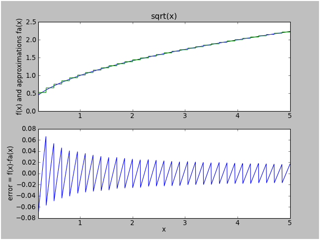
Note the stairsteppy result and the sawtooth error plot. This is typical for a plain table approach. The maximum error is roughly proportional to the slope of the function within an interval (the error is larger for small values of x where \( \sqrt{x} \) is steeper), and proportional to the interval size. If we want to reduce the error by a factor of 10, we need 10x as many lookup table entries.

If we want to improve the situation, the next improvement we can use is linear interpolation:

• At design time (or initialization time), divide the input range of the function into N intervals and evaluate the function at the N+1 endpoints of those intervals. (Usually the intervals are equal width)
• At runtime:
• handle out-of-range situations (either throw an error or return a value corresponding to min/max input)
• compute an index k of which interval the function is in
• lookup the value in the table at that index and the next index
• perform a linear interpolation: y = table[k]*(1-u) + table[k+1]*u, where u is the number between 0 and 1 representing the position of the input within the interval (0 = beginning of interval, 1 = end)

import math
def maketable1(func, a, b, n):
    table = func([float(x)/n*(b-a)+a for x in range(0,n+1)])
    def tablefunc(x):
        if x < a or x > b:
            raise "out of range error"
        ii = (x-a)/(b-a)*n
        i = math.floor(ii)
        if i == n:
            i = n-1
        u = ii-i
        return table[i]*(1-u) + table[i+1]*u
    return tablefunc
sqrtapproxf = maketable1(np.sqrt, 0.2, 5.0, 32)

Here's the error plot for approximation "f":

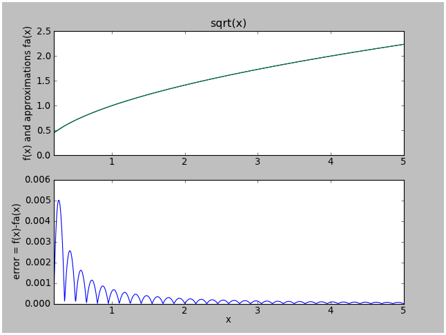
Much better — note the error plot containing parabolic sections. This is typical for interpolated table lookup. The maximum error is roughly proportional to the curvature (2nd derivative) of the function within an interval, and proportional to the square of the interval size. If we want to reduce the error by a factor of 10, we only need about 3x as many lookup table entries.

This is one of the rare cases where table interpolation may be more appropriate than polynomial evaluation: the maximum error here is about 1/2 as much as the 5th-order polynomial we used in approximation "d".

For a comparison in execution time: table lookup with no interpolation is roughly equivalent to a quadratic (2nd order) function, and table interpolation is roughly equivalent to a quartic (4th order) polynomial. That's only an estimate; it really depends on things like whether you're doing floating-point or fixed-point computation, whether the table has a length that is a power of 2 (it should be, so you can use bitwise operations to speed up the math), and how long it takes to perform table lookups on your processor.

There are only a few situations, in my opinion, where table lookup is appropriate:

• If accuracy requirements are very low, a non-interpolated table lookup may be sufficient.
• If a function is very "nonpolynomial" then an interpolated table lookup may produce superior accuracy compared to a polynomial evaluation of comparable execution time. (This appears to be the case for \( \sqrt{x} \) over the \( [0.2, 5.0] \) range. We'll define "nonpolynomial" shortly; for now just think of it as a function with a lot of wiggles or twists and turns.)
• If a function is very difficult to approximate with a polynomial over the whole range but needs very high accuracy, one option is to split the range into 4 or 8 subintervals and use table lookup to obtain polynomial coefficients for each subinterval.

Table lookup is not appropriate when it requires such a large table size that you have to worry about memory requirements.

Also note that the error in approximation "f" is not fairly distributed: the maximum error happens at the low end of the input range and is much smaller over the rest of the input range. You can use tricks to make the error distribution more fair, namely by using variable-width intervals, but there's no general process for doing this while still using an efficient computation at runtime.

Chebyshev Polynomials

The key to using polynomials to evaluate functions, is not to think of polynomials of being composed of linear combinations of \( 1, x, x^2, x^3 \), etc., but as linear combinations of Chebyshev polynomials \( T_n(x) \). As discussed in more detail in the Wikipedia page, these have the following special properties:

• they are minimax functions over the range \( [-1,1] \), e.g. all their minima/maxima/extrema are at ± 1 (see diagram below)
• they are orthogonal over the range \( [-1,1] \) with weight \( \frac{1}{\sqrt{1-x^2}} \)
• \( T_0(x) = 1, T_1(x) = x, T_{n+1}(x) = 2xT_n(x) - T_{n-1}(x) \)
• \( T_n(x) = \cos(n \cos^{-1} x) \)

Figure: Chebyshev functions \(T_n(x)\), courtesy of Wikipedia

Let's say we have a given function \(f(x)\) over the range \( x \in [a,b] \). We can express \( f(x) = \sum c_k T_k(u) \) where \( u = \frac{2x-a-b}{b-a} \) and \( x = \frac{b-a}{2}u + \frac{a+b}{2} \), which is a transformation which maps the interval \( x \in [a,b] \) to \( u \in [-1,1] \). The problem then becomes a matter of figuring out the coefficients \( c_k \), which can be done using the Chebyshev nodes:

These are easier to understand graphically; they are merely the projections onto the x-axis of the midpoints of equal interval circular arcs of a semicircle:

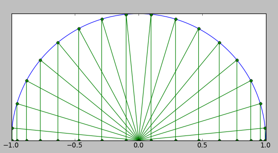
You will note that the nodes are spaced equally near 0 and more compressed towards ± 1.

To approximate a function by a linear combination of the first N Chebyshev polynomials (k=0 to N-1), the coefficient \( c_k \) is simply equal to \( A(k) \) times the average of the products \( T_k(u)f(x) \) evaluated at the N Chebyshev nodes, where \( A = 1 \) for \( k = 0 \) and \( A = 2 \) for all other k.

Let's illustrate the process more clearly with an example.

Suppose \( f(x) = \frac{1}{3} x^3 + 2x^2 + x - 10 \) over the range \( [-1, 3] \), with \( u = \frac{x-1}{2}, x = 2u+1 \):

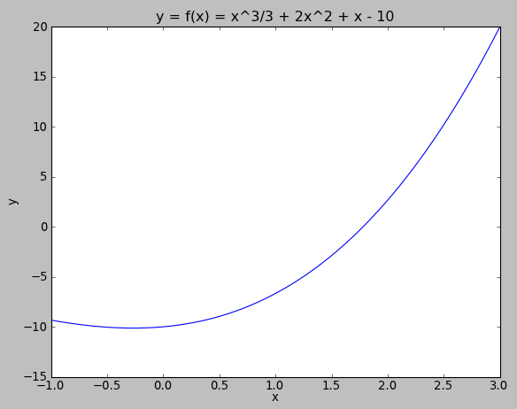
Let's use \( N=5 \). The Chebyshev nodes for N=5 are \( u=-0.951057, -0.587785, 0, +0.587785, +0.951057 \). This corresponds to \( x=-0.902113, -0.175571, 1, 2.175771, 2.902113 \), and the function \( f(x) \) evaluated at those nodes are \( y=-9.51921, -10.11572, -6.66667, 5.07419, 17.89408 \).

For \( c_0 \) we compute the average value of y = \( (-9.51921-10.11572-6.66667+5.07419+17.89408)/5 = -0.66667 \).

For \( c_1 \) we compute 2 × the average value of u × y = \( 2\times(-9.51921\times-0.951057+-10.11572\times-0.587785\) \(+-6.66667\times 0+5.07419\times 0.587785+17.89408\times 0.951057) = 14 \)

For \( c_2 \) we compute 2 × the average value of \( T_2(u)\times y = (2u^2-1) \times y \: \longrightarrow \: c_2 = 6 \)

For \( c_3 \) we compute 2 × the average value of \( T_3(u)\times y = (4u^3-3u) \times y \: \longrightarrow \: c_3 = 0.66667\)

For \( c_4 \) we compute 2 × the average value of \( T_4(u)\times y = (8u^4-8u^2+1) \times y \: \longrightarrow \: c_4 = 0 \)

The conclusion here is that \( f(x) = -\frac{2}{3}T_0(u) + 14T_1(u) + 6T_2(u) + \frac{2}{3}T_3(u) \) ; if you go and crunch through the algebra you will see that the result is the same as \( f(x) = \frac{1}{3}x^3 + 2x^2 + x - 10 \).

So what was the point here....? Well, if you already have the coefficients of a polynomial, there's no point in using Chebyshev polynomials. (If the input range is significantly different from \( [1,1] \), a linear transformation from x to u where \( u \in [-1,1] \) will give you a polynomial in u that has better numerical stability, and Chebyshev polynomials are one way to do this transformation. More on this later) If you want to approximate the polynomial with a polynomial of lesser degree, Chebyshev polynomials will give you the best approximation.

For example let's use a quadratic function to approximate \( f(x) \) over the input range in question. All we need to do is truncate the Chebyshev coefficients: let's compute $$\begin{eqnarray} f_2(x) &=& -\frac{2}{3}T_0(u) + 14T_1(u) + 6T_2(u) \cr &=& -\frac{2}{3} + 14u + 6\times(2u^2-1) \cr &=& -\frac{20}{3} + 14u +12u^2 \cr &=& -\frac{20}{3} + 7(x-1) + 3(x-1)^2 \cr &=& 3x^2 + x - \frac{32}{3}. \end{eqnarray} $$

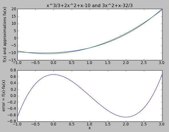
Voila! We have a quadratic function that is close to the original cubic function, and the magnitude of the error is just the coefficient of the Chebyshev polynomial we removed = \( \frac{2}{3} \).

You will note that these two polynomials (\( \frac{1}{3}x^3 + 2x^2 + x - 10 \) and \( 3x^2 + x - \frac{32}{3} \)), expressed in their normal power series form, have no obvious relation to each other, whereas the Chebyshev coefficients are the same except in coefficient \( c_3 \) which we set to zero to get a quadratic function.

In my view, this is the primary utility of expressing a function in terms of its Chebyshev coefficients: The coefficient \( c_0 \) tells you the function's average value over the input range; \( c_1 \) tells you the function's "linearness", \( c_2 \) tells you the function's "quadraticness", \( c_3 \) tells you the function's "cubicness", etc.

Here's a more typical and less trivial example. Suppose we wish to approximate \( \log_2 x \) over the range \( [1,2] \).

A decomposition into Chebyshev coefficients up to degree 6 yields the following:

$$\begin{eqnarray} c_0 &=& +0.54311 \cr c_1 &=& +0.49505\cr c_2 &=& -0.042469\cr c_3 &=& +0.0048577\cr c_4 &=& -6.2508\times 10^{-4}\cr c_5 &=& +8.5757\times 10^{-5}\cr c_6 &=& -1.1996\times 10^{-5}\cr \end{eqnarray} $$

You will note that each coefficient is only a fraction of the magnitude of the previous coefficient. This is an indicator that the function in question (over the specified input range) lends itself well to polynomial approximation. If the Chebyshev coefficients don't decrease significantly by the 5th coefficient, I would classify that function as "nonpolynomial" over the range of interest.

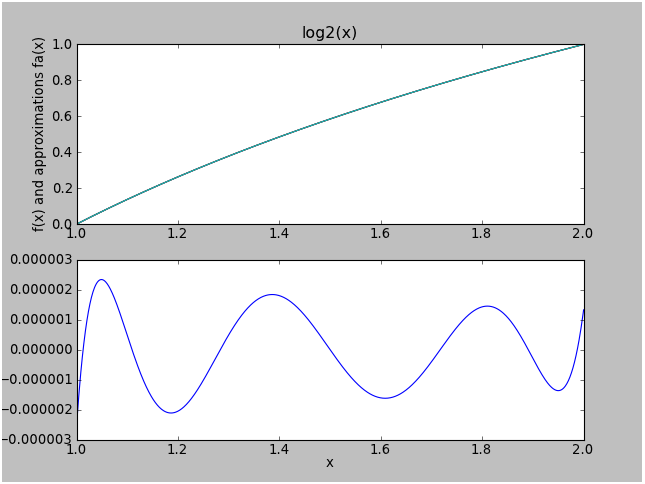
The maximum error for the 6th-degree Chebyshev approximation for \( \log_2 x \) over \( x \in [1,2] \) is only about 2.2×10^-6, which is approximately the value of the next Chebyshev coefficient.

If we truncate the series to a 4th-degree Chebyshev approximation, we get a maximum error that is about equal to \( c_5 = 8.6×10^{-5} \):

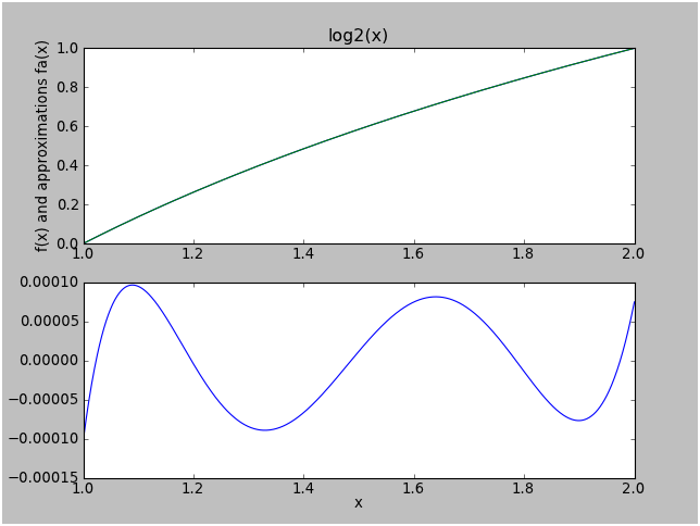
Neat, huh?

Some further examples of elementary functions

Here is a list of common functions, along with the first 6 Chebyshev coefficients:

\( f(x) \)	range	c0	c1	c2	c3	c4	c5
\( \sin \pi x \)	[-0.5,0.5]	0	1.1336	0	-0.13807	0	0.0045584
\( \sin \pi x \)	[-0.25,0.25]	0	0.72638	0	-0.01942	0	0.00015225
\( \cos \pi x \)	[-0.5,0.5]	0.472	0	-0.4994	0	0.027985	0
\( \cos \pi x \)	[-0.25,0.25]	0.85163	0	-0.14644	0	0.0019214	0
\( \sqrt{x} \)	[1,4]	1.542	0.49296	-0.040488	0.0066968	-0.0013836	0.00030211
\( \log_2 x \)	[1,2]	0.54311	0.49505	-0.042469	0.0048576	-0.00062481	8.3994e-05
\( e^x \)	[0,1]	1.7534	0.85039	0.10521	0.0087221	0.00054344	2.7075e-05
\( \frac{2}{\pi}\tan^{-1} x \)	[-1,1]	0	0.5274	0	-0.030213	0	0.0034855
\( \frac{1}{1 + e^{-x}} \)	[-1,1]	0.5	0.23557	0	-0.0046202	0	0.00011249
\( \frac{1}{1 + e^{-x}} \)	[-3,3]	0.5	0.50547	0	-0.061348	0	0.01109
\( \frac{1}{1 + x^2} \)	[-1,1]	0.70707	0	-0.24242	0	0.040404	0
\( \frac{1}{1 + x^2} \)	[-3,3]	0.30404	0	-0.29876	0	0.12222	0

Other comments

A great reference for Chebyshev functions is Numerical Recipes by Press, Teukolsky, Vetterling, and Flannery, which covers Chebyshev approximation in detail.

There are a few things to note when evaluating Chebyshev functions:

• It's better to compute the functions directly rather than trying to convert Chebyshev approximations to a standard polynomial form. (that is, if you want to calculate \( 3T_0(x) + 5T_1(x) - 0.1T_2(x) \) , don't convert to a polynomial, but instead calculate the T values directly.) Numerical Recipes recommends Clenshaw's recurrence formula, but I just use the following simple algorithm:

u = (2*x-a-b)/(b-a)
Tprev = 1
T = u
y = c[0]
for i = 1:n
    y=y+T*c[i]
   Tnext = 2*u*T - Tprev
   Tprev = T
   T = Tnext

• Remember to convert from x to u — this keeps the numerical stability of the algorithm, because polynomials tend to be well-conditioned for evaluating arguments between -1 and 1, and ill-conditioned for arguments with very large or very small magnitudes.

Here is a Python class for computing and applying Chebyshev coefficients:

import math
import numpy as np
def chebspace(npts):
    t = (np.array(range(0,npts)) + 0.5) / npts
    return -np.cos(t*math.pi)
def chebmat(u, N):
    T = np.column_stack((np.ones(len(u)), u))
    for n in range(2,N+1):
        Tnext = 2*u*T[:,n-1] - T[:,n-2]
        T = np.column_stack((T,Tnext))
    return T
class Cheby(object):
    def __init__(self, a, b, *coeffs):
        self.c = (a+b)/2.0
        self.m = (b-a)/2.0
        self.coeffs = np.array(coeffs, ndmin=1)
    def rangestart(self):
        return self.c-self.m
    def rangeend(self):
        return self.c+self.m
    def range(self):
        return (self.rangestart(), self.rangeend())
    def degree(self):
        return len(self.coeffs)-1
    def truncate(self, n):
        return Cheby(self.rangestart(), self.rangeend(), *self.coeffs[0:n+1])
    def asTaylor(self, x0=0, m0=1.0):
        n = self.degree()+1
        Tprev = np.zeros(n)
        T     = np.zeros(n)
        Tprev[0] = 1
        T[1]  = 1
        # evaluate y = Chebyshev functions as polynomials in u
        y     = self.coeffs[0] * Tprev
        for co in self.coeffs[1:]:
            y = y + T*co
            xT = np.roll(T, 1)
            xT[0] = 0
            Tnext = 2*xT - Tprev
            Tprev = T
            T = Tnext
        # now evaluate y2 = polynomials in x
        P     = np.zeros(n)
        y2    = np.zeros(n)
        P[0]  = 1
        k0 = -self.c/self.m
        k1 = 1.0/self.m
        k0 = k0 + k1*x0
        k1 = k1/m0
        for yi in y:
            y2 = y2 + P*yi
            Pnext = np.roll(P, 1)*k1
            Pnext[0] = 0
            P = Pnext + k0*P
        return y2
    def __call__(self, x):
        xa = np.array(x, copy=False, ndmin=1)
        u = np.array((xa-self.c)/self.m)
        Tprev = np.ones(len(u))
        y = self.coeffs[0] * Tprev
        if self.degree() > 0:
            y = y + u*self.coeffs[1]
            T = u
        for n in range(2,self.degree()+1):
            Tnext = 2*u*T - Tprev
            Tprev = T
            T = Tnext
            y = y + T*self.coeffs[n]
        return y
    def __repr__(self):
        return "Cheby%s" % (self.range()+tuple(c for c in self.coeffs)).__repr__()
    @staticmethod
    def fit(func, a, b, degree):
        N = degree+1
        u = chebspace(N)
        x = (u*(b-a) + (b+a))/2.0
        y = func(x)
        T = chebmat(u, N=degree)
        c = 2.0/N * np.dot(y,T)
        c[0] = c[0]/2
        return Cheby(a,b,*c)

You can put this in a file cheby.py and then use it as follows (here we fit \( \sin x \) between 0 and \( \frac{\pi}{2} \) with a 5th degree polynomial, and compute our approximation on angles 0, \( \frac{\pi}{6} \), \( \frac{\pi}{4} \), and \( \frac{\pi}{3} \)):

>>> import cheby
>>> import numpy as np
>>> import math
>>> c = cheby.Cheby.fit(np.sin,0,math.pi/2,5)
>>> c
Cheby(0.0, 1.5707963267948966, 0.60219470125550711, 0.51362516668030367, -0.10354634422944738, -0.013732035086651754, 0.001358650338492214, 0.00010765948465629727)
>>> c(math.pi*np.array([0, 1.0/6, 1.0/4, 1.0/3]))
array([  6.21628624e-06,   5.00003074e-01,   7.07099696e-01,
         8.66028717e-01])

Function approximation for empirical data

Let's go back to the beginning of our discussion to Bill's problem. He has a nonlinear sensor relating a physical quantity (gas concentration) to a voltage measurement; the problem he faces is how to invert that relation so that he can estimate the original physical quantity: \( y = f(x) \) where x is the measurement and y is the physical quantity.

Chebyshev approximation works well here too, but we have a problem. We can't just evaluate \( f(x) \) at Chebyshev nodes to get the Chebyshev coefficients, because we don't know for certain what \( f(x) \) actually is. Instead, we have to make some reference measurements to determine those coefficients, with known physical quantities (e.g. known gas concentrations in Bill's case), and tabulate these x and y values, then use them to estimate the coefficients. We have two choices in selecting the measurements:

• Try to plan the measurements so that the values x lie near the Chebyshev nodes over the expected range. This will allow us to use fewer measurements.
• Make a lot of measurements so the whole input range is well-covered

In some situations, it's quick and easy to make measurements with arbitrary references. (For example, if you're trying to calibrate a microphone, you can change the amplitude and frequency of reference sound signals automatically with electronic equipment), and the second option is a viable one. In other situations, like the gas concentration problem, it may be inconvenient or expensive to make lots of measurements, and you have to select the reference values carefully.

The best way I've found to estimate Chebyshev coefficients from empirical data, is to use weighted least-squares:

• Collect the measurements x and physical input quantity y into vectors X and Y
• For the vector of measurements x, compute u from x, and compute the values of the Chebyshev polynomials \( T_0(u), T_1(u), T_2(u), \ldots T_n(u) \) and save each these as vectors in a matrix T. Each polynomial will be used as a basis function.
• Compute a weighting value \( w(x) \) to compensate for the density of values x. (e.g. if lots of x values are near \( x=0 \) but very few of them are near \( x=1 \), you may have to choose \( w(x) \) low near \( x=0 \) and higher near \( x=1 \) .) Express these values as a diagonal matrix W.
• Compute a vector C of coefficients \( c_0, c_1, c_2, \ldots c_n \) using weighted least-squares to solve for C:
  $$(T^TWT)C = T^TWY.$$ To do this you will need some kind of matrix library. In MATLAB this would be computed as C = (T'*diag(W)*T)\(T'*diag(W)*Y). In Python with Numpy, you can skip calculating the T matrix, and just use the numpy.polynomial.chebyshev.chebfit function on the x and y measurements; the weighting vector is an optional input.

I would not use a degree greater than 5. If you find you're still not getting a good approximation with a 5th degree polynomial, you're probably using the wrong approach; the function is too sharp or wiggly or cusped. Higher degree polynomials can have problems with numerical accuracy.

In any case, function approximation of empirical data is a little trickier than approximation of known functions. Always make sure you double-check your approximation by graphing the original data and the function you come up with.

Wrapup

The next time you need to turn to function approximation, give Chebyshev approximation a shot! Not only is it probably the best and easiest way to approximate a function with a polynomial, but it will also let you know how well polynomials approximate the function in question, by the behavior of the Chebyshev coefficients.

Make sure you choose the required accuracy and input range of your function wisely. Too high of an accuracy and too wide an input range will require higher degrees of polynomials and longer execution times, and high degree polynomials are often numerically ill-conditioned.

More efficient evaluation of functions will mean you can use less CPU resources for a desired accuracy. So this can save you money and influence your coworkers.

Happy approximating!

---

© 2012 Jason M. Sachs, all rights reserved.

y = y * x + c

Sign in