Some Observations on Comparing Efficiency in Communication Systems

• Wireless
• Communication

Introduction

Engineering is usually about managing efficiencies of one sort or another. One of my favorite working definitions of an engineer says, "An engineer is somebody who can do for a nickel what any damn fool can do for a dollar." In that case, the implication is that the cost is one of the characteristics being optimized. But cost isn't always the main efficiency metric, or at least the only one. Consider how a common transportation appliance, the automobile, is optimized differently for the different applications listed below:

1. A consumer commuter vehicle that also serves as domestic family transportation.
2. An urban taxi cab.
3. A race car that runs laps on a road course.
4. A race car that competes for the minimum elapsed time on a quarter-mile drag strip.

Even though all of those examples will produce something recognizable as a "car", the differences due to the optimizations will be huge. Even for the subclass of "race car", a road race car is optimized completely differently than a straight-line drag car and neither will perform competitively in a satisfactory manner at the other's task.

So the optimization or efficiency criteria for a system have a big affect on how that system might be engineered. Communication systems are no different, and certain resources may be more or less precious and certain impairments be more or less cumbersome from application to application. For a communication system two important characteristics that often drive the system design are transmit power efficiency and spectral efficiency. These two characteristics are often mutually exclusive and interrelated at the same time. In this article we will explore some of the tradeoffs around these two metrics and make some observations about their impacts on system design.

Resource Management

Optimization of efficiencies in systems is usually about resource management. Cost is almost always a consideration, in that cost should be minimized or managed, because the money available to pay for the result is limited and can be used for other things if savings are made. In communication systems transmit power and channel spectrum are often resources that have to be managed. Depending on the application, power may be more or less of a concern, and likewise with channel spectrum. Whichever resource is the most precious may dictate whether the system leans toward a design optimized for power efficiency or for spectral efficiency.

Systems for which maximizing usable range is important require high power efficiency. The characteristics of the Power Amplifier (PA) in the transmitter may also drive requirements around power efficiency. The PA is often the largest consumer of electrical power in a transmitter, even in something small and highly integrated like a cellular handset. If long battery life is a concern, then maximizing the efficiency of the transmitted power can help extend battery life. The PA is also often one of the more expensive components in a system, and cost is often proportional to output power, so minimizing the amount of transmit power needed, by increasing power efficiency, can directly reduce the cost of the transmitter. So some systems that may not require maximum range may still want to achieve high power efficiency in order to extend battery life or to reduce transmitter cost. A good example of an extreme case where power efficiency is important is a deep-space probe, like the exploration vehicles sent out to gather data about the other planets in the solar system or various comets or asteroids. Since their range requirements are extreme, and their available power is limited, squeezing every bit of efficiency out of the available transmit power is useful.

In some situations the available spectrum may be a valuable resource that needs to be managed. For certain applications where licensed spectrum is allocated to specific users, and where more bandwidth is available than needed, spectral efficiency may not be too important. In many applications, however, and the number is growing all the time as demand for streaming data increases, it is desirable to squeeze as much data or as many signals as possible into an available channel in a certain chunk of spectrum. Networked systems that allow multiple users to access the channel, like cellular, cable, or WiFi systems, can minimize the time or bandwidth required by each user if the spectral efficiency of the user's transmissions are increased. This relieves network traffic congestion and allows the network to operate more smoothly.

Most systems need some combination or mix of power efficiency and spectral efficiency. Satellite networks need power efficiency to close the link at the long ranges required, and the satellite transponders have limited bandwidth. Likewise cellular systems must be able to manage both spectral efficiency to meet high throughput demands by multiple users, but also power efficiency when users are at the edge of a cell's coverage area and to extend handset battery life.

Efficiency Metrics and Management

Quantitative analysis of efficiency requires suitable metrics. For power efficiency the usual metrics for digital systems quantify reliability, or probability of error, with respect to a relevant measure of the power required to transmit the data. For continuous-stream systems, like video transport or backhaul systems, the Bit Error Rate (BER) provides a good reliability metric. For bursty or packet transmission systems, the Packet Error Rate (PER) or Block Error Rate (BLER) is often used, where a representative packet or block size is specified. Once the reliability metric is determined the power efficiency can be evaluated by measuring the reliability against the received power. Since the thermal noise floor is essentially a constant for a given receiver at operating temperature (thanks to Boltzmann's constant), as the received power goes down the received SNR goes down. For a continuous data stream system that uses BER as the reliability metric, the SNR can be converted to E_b/N_o, or energy-per-bit over noise power in a unit-Hz bandwidth. E_b/N_o is a handy metric, since relating the Bit Error Rate to bit energy is useful, but also because it allows different Forward Error Correction (FEC) code rates and modulations to be compared independent of the system bandwidths in a relevant way. For systems using PER as the reliability metric, comparison against SNR or C/N is more common since bursty or packet systems typically use the same bandwidth regardless of modulation or FEC code rate (e.g., WiFi). E_b/N_o normalizes the power ratio as though the data rate were held constant, so that the transmission technique, specifically the modulation and FEC performance, can be evaluated in terms that reflect the power efficiency relative to the payload data. SNR, on the other hand, is more suitable for cases where the transmit power and signal bandwidth are constant and the data rate varies as the modulation and code rate are changed. This difference is subtle but important in evaluating system performance.

Metrics for spectral efficiency are more straightforward, usually being expressed as payload bits per second per Hertz (bits/s/Hz) or throughput, for channels with fixed bandwidth. The payload bit rate is the net information rate after the overhead due to the FEC code rate is accounted for, and usually after other overhead such as guard intervals or guard bands are taken into consideration.

Basic Performance Characterization

Figure 1 shows an ensemble of common modulation types and code rates for a single-carrier Trellis Coded Modulation (TCM) system with Convolutional Coding (CC) concatenated with an outer Reed-Solomon (RS) code and with Viterbi-Reed-Solomon (Vit-RS) decoding. Since the performance curves are shown as BER vs E_b/N_o, only power efficiency relative to the payload data is depicted. The same plot can be rescaled and plotted against SNR instead of E_b/N_o, as in Figure 2. Doing so then compares performance as a function of total transmitted power rather than information bit energy. This changes the dependence on spectral efficiency since the noise bandwidth relative to the data rate (and therefore E_b, the energy per payload bit) changes as the modulation and code rate change. It can be seen that some of the relative performance comparisons change, which is especially noticeable between the 64-QAM R = 3/4 and R = 5/6 cases. This suggests that a system engineer may wish to make a different Modulation and Coding Scheme (MCS) selection tradeoff depending on whether payload information transmission efficiency or link margin or total transmit power or some other metric is the most important.

Systems that make use of Adaptive Coding and Modulation (ACM) are often evaluated using throughput plots when determining adaptation strategies. In this case the system bandwidth is typically fixed, as is often the transmit power. This means that the adaptation across the MCS set trades throughput for reliability which is often described as trading rate for range. In this case SNR is used instead of E_b/N_o since the resources, specifically the signal bandwidth and transmit power, are fixed and the desire is to obtain the maximum throughput reliably allowed by the channel under varying channel conditions. Generally such throughput evaluations are done using packet or block statistics since adaptation requires a return channel which also means that Automatic Repeat reQuest (ARQ) retransmission of failed packets is also possible. Figure 3 shows an example throughput vs SNR curve ensemble for an 802.11a WiFi system. Throughput is computed by the maximum throughput of each MCS set scaled by 1-PER.

The information shown in an ensemble of throughput curves, like that shown in Figure 3, can be used to develop adaptation strategies by observing the MCS selection that provides the maximum throughput for a given channel condition. The strategy selected may differ depending on system constraints, the type of traffic carried, or other factors. For example, if a low PER is desired in order to minimize retransmissions (which further reduce throughput) and latency, the lower-order MCS selections will tend to be used more heavily in order to maximize reliability at the expense of some overall throughput. Whatever strategy is used, the system can trade rate for reliability (or range, depending on how one wants to look at it), by reducing the order of the MCS selection as the channel deteriorates. This is an adaptive efficiency optimization process that makes use of the differences in power efficiency between various MCS selections.

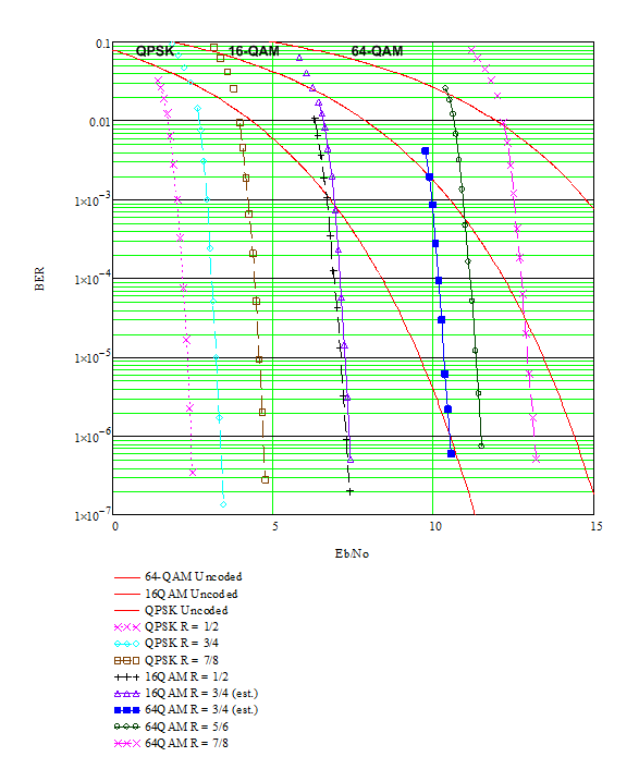
Figure 1, BER vs E_b/N_o performance curves for various example modulations and code rates. These curves are for TCM in AWGN with concatenated Viterbi-Reed-Solomon (Vit-RS) decoding. The matched-filter bound curves for each modulation, QPSK, 16-QAM, and 64-QAM, with grey coding are shown as solid red traces.

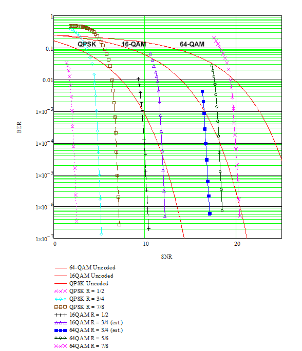
Figure 2. This is essentially Figure 1 with the horizontal axis rescaled to show SNR rather than E_b/N_o. Sometimes the relative performance gains change when the comparison changes between E_b/N_o and SNR. Note that the relative performance difference between the 16QAM and 64QAM schemes have changed from Figure 1.

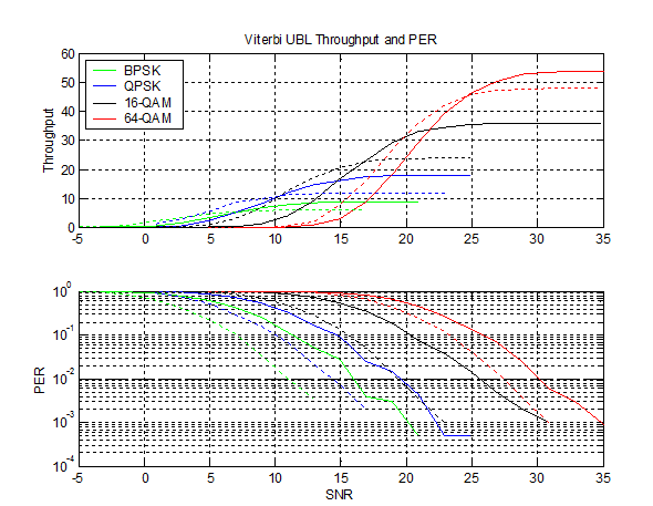
Figure 3. Example throughput curves for an 802.11a WiFi system in multipath fading (IEEE 802.11n Channel Model D, 50ns delay spread) and noise. Throughput is calculated as the maximum rate for each MCS selection times 1-PER for that MCS selection. The different code rates for each modulation type are shown as dashed or solid lines for each modulation-specific color. Channel adaptation strategies can be evaluated using this sort of throughput analysis. (This figure is from a presentation made by Intel to the IEEE 802.11n Working Group based on work done at Intel's Nizhny Novgorod Laboratory.)

Analyzing Efficiency from Performance Data

It should be noted that often multiple system characteristics come into play when evaluating performance and efficiency for a wireless system. In Figs. 1 and 2 the MCS set performance is shown in AWGN. In Fig. 1 E_b/N_o is used in the horizontal axis which means the FEC and modulation performances can be compared strictly in a data power efficiency sense. In Fig. 2 SNR is used which changes the relative positions of the curves from Fig. 1 slightly. Figure 3 compares throughput against SNR in frequency-selective multipath fading, so the performance of the MCS selections and any channel interleavers or other channel-mitigation processing may also be included. In many cases, like that shown in Fig. 3, it is important to understand whether channel estimation and synchronization effects are also included. Often it will be stated whether perfect synchronization and channel knowledge are used in simulations, which was the case for Fig. 3. This allows separation of comparison of either just the MCS set or other system processing like synchronization, channel estimation, and equalization.

Comparison against theoretical bounds is a useful tool for maximizing things like power efficiency, and theoretical channel capacity limits are often used for comparing things like FEC performance. Figures 1 and 2 show the theoretical matched filter bounds for uncoded performance of the indicated modulation schemes, and these are generally used to measure the coding gain of FEC solutions. "Coding Gain" is the improvement in power efficiency that a FEC system provides compared to the matched-filter bound uncoded performance, and is often shown on a BER vs E_b/N_o plot in order to assess the performance of the FEC system. While the matched filter bound is a reference point on the low-efficiency end of the scale, channel capacity is a theoretical limit of the highest power efficiency possible for information transmission. It is often useful to compare a system's performance against the theoretical channel capacity in order to judge how much performance can be improved.

Figure 4 shows a comparison of three FEC systems, a common Convolutional Code (CC) (decoded with a Viterbi decoder) with an outer Reed-Solomon (RS) code with rate R = 3/4 (four transmitted bits for every three information payload bits), a Parallel Concatenated Convolution Code (PCCC) Turbo Code (TC) with an outer Reed-Solomon (RS) code with rate R = 3/4, and a related PCCC TC-RS with R = 9/10. The matched filter bound for QPSK is shown in the solid red trace and the theoretical channel Capacity (C) is shown for both an R = 3/4 and an R = 9/10 code using QPSK. Channel Capacity is the theoretical limit of SNR (or E_b/N_o) below which reliable communications cannot be made. Usually this is stated as the boundary above which error-free communications can be made, but it boils down to essentially the same thing. The coding gain and distance to capacity are shown for the R = 3/4 Vit-RS and the R = 9/10 TC-RS codes. An interesting observation is that at first glance the Vit-RS code appears to be superior in a strict power-efficiency sense, since it is to the left of the R = 9/10 TC-RS curve. The coding gain for the Vit-RS code is higher than it is for the R = 9/10 code. Since only power efficiency is shown on this plot the bandwidth advantage of the R = 9/10 code, due to the higher code rate, is not taken into account. A hint can be gleaned from the fact that the distance to capacity, shown in the vertical dashed red trace, is much less for the R = 9/10 TC-RS code than it is for the Vit-RS decoder. This suggests that the R = 9/10 code is a more powerful code than the Vit-RS system. The R = 3/4 TC-RS curve is shown as a reference to verify that the TC-RS system is superior to the Vit-RS at the same code rate.

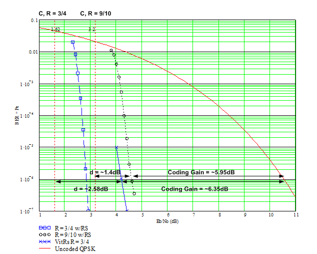
Figure 4. Shown is a comparison of three codes, an R = 3/4 concatenated convolution and Reed-Solomon (RS) code (decoded with a Viterbi-RS decoder), and two Parallel Concatenated Convolutional Code (PCCC) Turbo Codes (TC) with an outer RS code of rates R = 3/4 and R = 9/10. Although the R = 3/4 Vit-RS performance is better in a power efficiency sense than the R = 9/10 TC-RS system, the Turbo Code is closer to capacity. Since the BER vs E_b/N_o curve shows only power efficiency, the improved spectral efficiency of the R = 9/10 code is not obvious.

Another way to compare "efficiency" is with the so-called "bandwidth-efficiency" plane. This plotting technique separates power efficiency and spectral efficiency into the two orthogonal axes of the plot. The horizontal axis is E_b/N_o (typically in dB), which shows power efficiency only, and the vertical axis is Spectral Efficiency in bits/sec/Hz. The Continuous-Input Continuout-Output (CICO) Capacity curve is usually included as a reference line for the "quality" of the systems being compared. This plotting technique allows power efficiency, spectral efficiency, and distance to CICO Capacity to be compared on a single plot. CICO Capacity is not specific to a particular modulation type and is generally plotted against E_b/N_o rather than SNR. Figure 5 shows a "bandwidth-efficiency" plot of the codes compared in Figure 4 at a BER of Pe = 10-6.

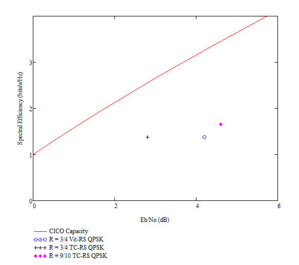
Figure 5. Bandwidth-Efficiency plane showing the codes compared in Figure 4 at a BER of Pe = 10-6. Power efficiency can be compared along the horizontal axis and bandwidth- or spectral-efficiency along the vertical axis. Generally systems that appear toward the upper left jointly utilize power and bandwidth more efficiently.

If the horizontal axis of Figure 5 is plotted as SNR rather than E_b/N_o, which requires rescaling for both code rate and modulation order, then CICO Capacity is generally replaced by Binary-Input Continuous-Output (BICO) Capacity that is specific to the modulation type considered. This allows comparison of FEC codes within a modulation type to analyze the exploitation of that particular modulation's BICO Capacity curve. Figure 6 shows the comparisons in Figure 5 replotted with SNR along the horizontal axis. It becomes more apparent in Figure 6 that for QPSK the R = 3/4 and R = 9/10 TC-RS codes operate closer to the BICO Capacity curve than the R = 3/4 Vit-RS system.

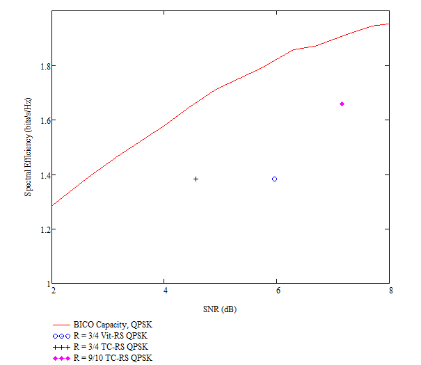
Figure 6. This is Figure 5 replotted against SNR rather than E_b/N_o and the CICO Capacity curve replaced by the BICO Capacity curve for QPSK. It is more evident here than in Figure 5 that the R = 9/10 TC-RS code operates closer to capacity than the R = 3/4 Vit-RS system.

It is possible to plot BICO capacities for a variety of modulation types and compare modulation and FEC combinations across an ensemble of MCS candidates. Information from plots like those shown in Figures 2 and 3 can be plotted for a reliability level of interest and compared. Often for continuous-stream systems or point-to-point systems BER is more relevant, but for bursty or multiple-access systems PER or BLER is often used. Figure 7 shows a comparison of several MCS candidates with a variety of FEC systems across QPSK, 16-QAM, and 64-QAM. The MCS set shown in Figs. 1-2 is included as the SC TCM set, and three example, proprietary, iterative decoding systems are shown as well: a Turbo Code with an outer RS code (TC-RS), a Low-Density Parity Check (LDPC) code, and a Turbo Product Code (TPC). All of these codes are compared at a BER of Pe = 10-6. Some example estimated performance data for an 802.11a system, which uses only a Convolutional Code with a Viterbi decoder, is also shown for reference. The 802.11a data is not directly comparable to the other FEC systems since it is a bursty, OFDM, multiple access system and the data shown is extrapolated from PER performance in multipath channels. The data shown for the other MCS candidates is for single-carrier modulation in AWGN channels.

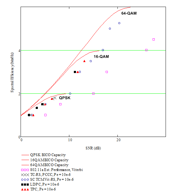
Figure 7. Spectral efficiency vs SNR for a number of Modulation and Coding Scheme candidates. Data is shown for TC-RS, TCM with concatenated CC-RS, LDPC and TPC FEC, all for single-carrier modulation in AWGN. Estimated performance data for an 802.11a OFDM WiFi system is also shown as a reference example.

It can be seen in most of the above plots that generally as SNR or E_b/N_o decreases, the modulation order and/or code rate must decrease in order to maintain link reliability. This tradeoff comes at the cost of spectral efficiency which usually means a decrease in throughput. In the plots showing spectral efficiency, specifically Figs. 5-7, higher power efficiency is on the left-hand side and higher spectral efficiency is toward the top of the plots. Joint optimization of both power and spectral efficiency means selecting MCS candidates toward the upper left as close to the capacity curves as possible. But where along the capacity curve should one operate? This is a system question that depends on many things, but an additional observation can be made by taking a closer look at Figure 6 as expanded in Figure 8. The shape of the BICO capacity curve is asymptotic to the number of bits/symbol of the modulation as SNR increases. This means that above a certain code rate, as the code rate increases performance would be expected to degrade much more quickly than at the low SNR end of the curve. This is labelled the Region of Diminishing Return for Coding in Figure 8. In order to operate in the left-most region of the curve spectral efficiency is reduced substantially as lower FEC code rates are required to maintain reliable reception of information. This is labelled the Region of Interest for Power Efficiency in Figure 8. This leaves the region near capacity around R = 0.75 - 0.9 as a sort-of "Sweet Spot" for operation that is reasonably both power and spectrum efficient.

The "Sweet Spot" shown in Figure 8 is notable not just for occupying the region of the capacity curve toward the upper-left corner of the plot. Capacity-approaching FEC codes like Turbo Codes, LDPC Codes, and Turbo-Product Codes tend to be fairly complex to implement. It is notable that in many architectures, and especially so for LDPCs and TPCs, the complexity goes down as the code rate goes up. Decoders built to operate with code rates in the R = 0.75 - 0.9 region will be, perhaps substantially, less complex than decoders built for lower code rates. This means that efficiency may be increased not only in utilization of transmit power and channel spectrum, but in cost and decoder power consumption as well. Also notable is the observation that, in general, known practical Turbo Product Codes, which typically can be realized with less complex decoders than TCs or LDPCs, operate closer to capacity at codes rates in the identified "Sweet Spot". For most systems, operating at extended range is an important requirement, and for systems with adaptive modulation it is important to have sufficient granularity in the MCS set for efficient adaptation strategies. These requirements will generally lead to population of lower code rates in order to make use of the Region of Interest for Power Efficiency shown in Figure 8. For some systems, however, where the optimization criteria allow it, it may be useful to exploit the joint efficiencies that may be realized by operating in the "Sweet Spot".

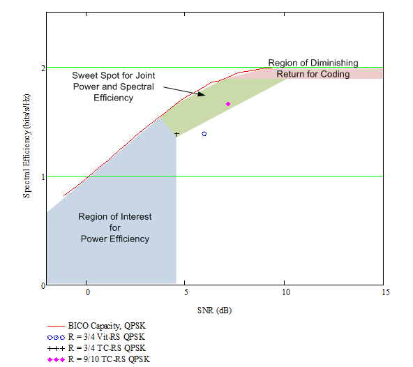
Figure 8. A close look at an expanded view of Figure 6 allows some observations about the nature of the typical modulation-specific BICO capacity curve. In this case the QPSK curve is divided into regions. In the left-most region Power Efficiency is optimized at the expense of spectral efficiency, and in the top-right region diminishing returns suggest code rates above about R = 0.9 are not useful. The remaining region near the capacity curve is then a "Sweet Spot" of sorts where Power Efficiency and Spectral Efficiency are high and decoder complexity and power consumption may be low.

Examples and Power Concentration

Interpretation of performance results as displayed in the different types of plots above requires attention to the system and application being analyzed. A couple of examples from the data shown previously may serve to illustrate some of the relevant points. Two systems will be considered: one a satellite link with a continuous fixed data-rate payload, like a digital video stream, and the other a multiple access wireless LAN system. An important distinction between the two is whether the channel bandwidth or the payload data rate is fixed.

In the example satellite system the payload data rate is fixed, which means that if the FEC code rate is changed to accommodate an equipment change (say, a different antenna with different gain) or a signal attenuation due to something like rain fade, the signal bandwidth will change when the code rate changes. Figure 9 illustrates the effect on signal power concentration due to the change in Power Spectral Density (psd) that results from the change in FEC code rate when the transmit power is held constant. An uncoded signal with no FEC will enjoy the highest power concentration, and therefore the highest SNR, since the symbol rate, and therefore the signal bandwidth, will be the minimum needed to support the required data rate. If a rate R = 1/2 FEC is added to improve reliability, the symbol rate, and therefore the signal bandwidth, doubles in order to support the FEC parity overhead added by the code. This reduces the PSD to half what it was in the uncoded case, and the SNR therefore drops 3 dB. Another way of looking at this is that the PSD of the noise floor is constant, with a unit-Hz density of N_o, so when the signal bandwidth doubles, the noise bandwidth, and therefore the noise power, also doubles. Even though the signal power is constant for both cases, the doubling of the in-band noise power when the signal bandwidth doubles reduces the SNR by 3 dB.

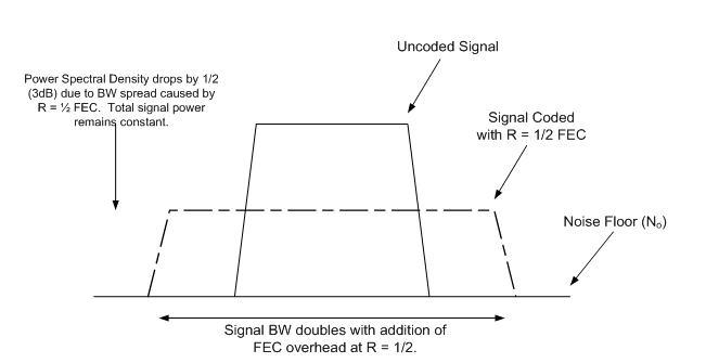
Figure 9. Changing the FEC code rate of a signal while holding the transmit power constant changes the Power Spectral Density by affecting the signal bandwidth. As the signal bandwidth increases the power spectral density drops and the in-band noise power increases.

The obvious question to ask at this point is why one would voluntarily take a 3 dB reduction in SNR to increase reliability? A quick glance back at Figure 1 shows that the difference between the uncoded QPSK (red, solid) curve and the R = 1/2 coded QPSK curve is about 8-9 dB at BER = 10-6. For the example satellite system with a fixed data rate and fixed transmit power E_b is fixed, and N_o is fixed by the noise temperature of the receiver, so E_b/N_o stays constant. Since Figure 1 is plotted against E_b/N_o, the 8-9 dB gain in effective power efficiency over an uncoded system already includes the effects of power concentration due to the different FEC code rates. So the 8-9 dB gain in performance is the net gain after the 3 dB drop due to the reduction in power concentration is accounted for.

For the wireless LAN case the signal bandwidth is fixed, so any change in FEC code rate will result in a change in the rate of the payload information that can be carried. If the transmit power is fixed and the signal bandwidth is fixed, the PSD, and therefore the SNR, is fixed and there is no reduction in power concentration. If the example shown in Figure 9 were repeated with the signal bandwidth held constant, the data rate would be cut in half when the R = 1/2 FEC was added to the uncoded signal. Cutting the data rate in half while the transmit power is held constant results in a doubling of E_b, the energy per payload bit.

Looking back at Figure 2, which is the system from Figure 1 plotted against SNR instead of E_b/N_o, the difference between the uncoded QPSK curve and the R = 1/2 coded QPSK curve is about 11-12 dB at BER = 10-6. The 3 dB difference in coding gain for the R = 1/2 QPSK case between Figs 1 and 2 is due to the power concentration (or dilution) effect of the R = 1/2 code rate. It must also be kept in mind that all of the signal power may not go to transmitting coded or uncoded payload information. It is not at all unusual for some transmit power to be allocated to pilot symbols or tones, frame markers, signalling information or other signal features that may be useful to the system that are transmitted along with the payload data. When E_b/N_o is used as a metric in performance analysis E_b is generally computed from the total transmit power, which means that there may also be a reduction in psd due to the additional bandwidth required for pilots or other signalling overhead. For the fixed signal-bandwidth case perspective, the SNR is not affected regardless of the overhead due to pilots or other signalling, only the data rate is reduced when bandwidth is consumed by other features. This results in the same increase in E_b seen in the fixed-bandwidth FEC case, since the reduced data rate due to either FEC parity or other overhead has the same effect. Many features that add overhead do not result in a measurable increase in performance (e.g., network protocol signalling), and may skew the performance curves. This emphasizes the point that care must be taken when evaluating performance curves to properly interpret the various effects on performance.

It can also be seen in Figs 1 and 2 that the 16-QAM R = 1/2 and R = 3/4 curves have nearly the same performance with respect to E_b/N_o (in Figure 1). This suggests that for the example fixed-data-rate satellite case there would be little advantage to switching between the two when adapting for changes in the system or the channel in such a system. However, in Figure 2 it can be seen that a gap of about 2 dB opens up between them at BER = 10-6 when plotted against SNR, as would be relevant for a fixed-channel-bandwidth system. For a fixed-bandwidth system the selection of 16-QAM R = 1/2 would provide an increase in power efficiency of about 2 dB over 16-QAM R = 3/4.

Separate from the nuances of interpreting performance with respect to E_b/N_o or SNR, the distance to capacity considerations illustrated in Figs. 4-8 generally also include the effects of modulation type and add the additional aspect of spectral efficiency. While Figs. 1 and 2 are useful in evaluating the performance of an MCS set as the SNR changes, Figs 4-8 provide tools for evaluating MCS candidates with respect to channel capacity in order to build an MCS set with the desired efficiency characteristics.

Conclusion

Like many things, improving "efficiency" in a wireless communication system requires deciding what characteristic of the system should be optimized. Evaluating efficiency for wireless communications is highly dependent on the nature of the system and the resource being optimized. Performance metrics may change between systems or between applications depending on whether streaming signals or bursty packets are used and whether the system is point-to-point or multiple access. The nature of the channel is also a significant consideration since performance in AWGN and fading channels are not easily comparable, and fading channels differ widely enough that care must be taken to make comparisons among like channels.

Optimizations for systems with Adaptive Coding and Modulation may be different from those without, and whether power or spectral efficiency is optimized may be system and application dependent. A general observation can be made that the shape of the typical modulation-specific BICO Capacity curve reveals a "Sweet Spot" that can be exploited using modern capacity-approaching codes. This sweet spot occupies a region at the knee of the curve that represents FEC code rates of, for example, around R = 0.75-0.9 for QPSK. Operating near capacity in this "sweet spot" provides efficient utilization of both power and spectrum bandwidth for those systems that can exploit it.

There is not a one-size-fits all approach to optimization or efficiency management for wireless systems. Squeezing the last bit out of various resources can easily hurt performance in other areas if one is not careful to understand the tradeoffs and operating space of the system. This article has touched on only a few areas from a few perspectives, and yet covers a wider range of efficiency aspects than many treatments of the topic. As wireless systems are asked to do a wider variety of tasks, rather than a single focused task, understanding these tradeoffs becomes more important.

References

[1] G. Ungerboeck, "Channel Coding with Multilevel/Phase Signals," IEEE Trans. Inform. Theory, vol. IT-28, No. 1, pp. 55-67, Jan. 1982.

Sign in