Update to a Narrow Bandpass Filter in Octave or Matlab

• Matlab

Following my earlier blog post (June 2020) featuring a Narrow Bandpass Filter, I’ve had some useful feedback and suggestions. This has inspired me to come up with an updated version, incorporating the following changes compared to the earlier one :

• Simpler code in Octave or Matlab
• Float32 precision replaces float64
• Faster processing by a factor of at least 4 times
• Easier setup of input parameters
• Normalized signal output level

A new experimental version in Python and Tensorflow running on Google Colab is also available here, more details at the end of this blog post.

OPERATION AND UPDATE DETAILS

For new readers, I suggest reading my previous blog which explained the theory of operation.  As a reminder, Figure 1 shows the basic configuration with complex down-conversion followed by baseband lowpass filtering and complex up-conversion.

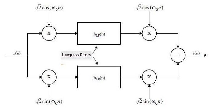
Fig 1. The basic filter with input signal x(n) and output y(n). [1]   Note that the sample rate throughout the filter remains constant.

Each of the two baseband filters of Figure 1 now has a single matrix IFIR filter followed by three identical RRS (moving sum) filters, each of length m1 (the IFIR expansion factor). The m1 expansion value is calculated automatically in the software. Note that the two baseband filters are identical.

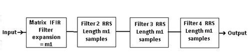
Fig 2.   Detail of a single lowpass baseband filter from Figure 1.

Filter design parameters include the number of taps and passband weight which are applied to the ‘remez’ filter design function (‘firpm’ may be used in Matlab). These function as for a conventional single stage filter, in that more taps give less passband ripple and higher stopband attenuation.The ‘weight_sb’ input parameter determines the ratio of stopband attenuation to passband ripple. Experimenting with both these values will give a useful feel for the capabilities of the filter.

The IFIR filter expansion value ‘m1’ is set by the software based on the sample frequency, number of taps, and the filter bandwidth.

The frequency response is illustrated using a chirp signal as the filter input. To obtain an accurate plot requires a minimum ‘signal block duration’ input parameter determined by the number of taps, and the passband.  Try using:   sbd = taps/(passband*2)   which gives 5 seconds for the example parameters of 10 Hz passband and 100 taps.

An external signal can replace the chirp test signal. This can have any of the following data formats:16, 24 or 32 bit unsigned integer, float32 or float64. Input data is converted to float32 for processing. The code has been tested with ‘.WAV’ files for input and output.

CODE WITH EXAMPLE PARAMETERS

Once again, the code listing below includes example parameters for a bandpass filter with a passband of 10 Hz and ripple less than 1 dB.  At a bandwidth of 13 Hz or greater the stopband attenuation exceeds 60 dB. Testing has been successful using a very wide range of sampling rates, bandwidths, and passband/stopband specifications.

The results in Figure 3 shows FFT plots generated using a filter with the example parameters. Running the code will also give a zoomed-in plot of the passband response.

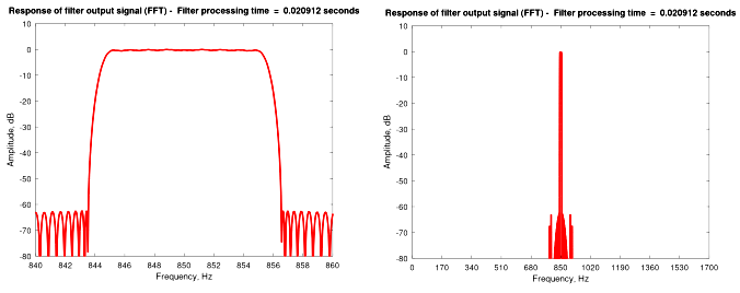
Fig 3.  Plots show filter frequency response after running the program in Octave with the example parameters from the code below.

CONCLUSION

The efficient bandpass filter described has been designed for easy implementation, and runs without modification in Octave version 6.1 or Matlab R2019b.

A new experimental version running Python and Tensorflow in Google Colab is also available here, which can be run by those of you with a Google account. To enable a GPU in Colab which considerably increases the processing speed :

Select :

• Menu> Runtime>Change runtime type.
• Change hardware acceleration to GPU.
• Click save.

I’m fairly sure the Tensorflow code could be made more efficient, in particular to make better use of the GPU.

Comments and suggestions for adapting and/or improving the code of either version are most welcome.

%
%               FIR narrow bandpass filter  ver 2.0
%               ===================================
%
%                     Paul Lovell   March 2021


   %   This program runs in Octave 6.1 using the 'remez' function
   %   (from the Octave-Forge 'signal' package), or in Matlab.
   %   It is an updated version of the design first published on
   %   dsprelated.com in June 2020.
   %   
   %   Specification for this bandpass filter example :
   %   Center frequency:                  850 Hz
   %   Passband:                          10 Hz at < 1dB
   %   Transition Region:                 13 Hz at > 60dB
   %   Sample rate:                       48 kHz
   %
   %   The taps in the first stage lowpass filter can be set 
   %   to any number > 30, as required. 
   %   Higher stopband attenuation, and/or a sharper transition
   %   band will require more taps.
   %   The weight of the stopband can also be increased or
   %   decreased relative to the passband. This results in 
   %   changes to passband ripple and stopband attenuation.
   %   
          
%  ***********************  Input Parameters  **********************
   
   %   Set the bandpass filter input parameters as required
      
   clear all;
   Fs = 48000;      %  Set sample rate in Hz
   passband = 10;   %  Set passband width Hz
   stopband = 13;   %  Set stopband limit Hz
   cfr = 850;       %  Set the center frequency
   taps = 100;      %  Set taps for first stage matrix IFIR filter
   sb_weight = 20;  %  Weight of stopband attenuation relative 
                    %  to passband ripple (passband weight = 1)
     
   %  Set the test signal duration in seconds as required. 
   %  The minimum value here is approx :  taps/(passband*2)
   %  (eg 5 seconds for a 10Hz passband filter with 100 taps)
   
   signal_block_drn = 5;           % test signal duration in seconds
        
   profile_on = false;
  
   %  The profile option works in Octave but may need to be
   %  changed for Matlab
  
                   
   psb = passband/2;
   stb = stopband/2;
   
   %  Test Chirp Signal input to the filter
   %  Replace this with your own input signal as required
   
   chfmin = 0;   chfmax = cfr * 2;
   dt = 1/Fs;    tw = (0:dt:signal_block_drn);
   
   sig = chirp(tw,chfmin,signal_block_drn,chfmax); 
   siglen = length(sig);


%%   % Enable this section for input from single channel .WAV file 
%%      
%%   [sig, Fs] = audioread("c:/dsp/input.wav"); % alternative input
%%   sig = sig'; siglen = length(sig);
%%   dt = 1/Fs; signal_block_drn = siglen/Fs;
%%   tw = (0:dt:signal_block_drn);
     
        
%  *****************  Down/up-conversion oscillators  *************  
  
   sinosc = single(sqrt(2) * sin(2*pi*cfr*tw));
   cososc = single(sqrt(2) * cos(2*pi*cfr*tw));
            
%  *******  Calculate filter passband and stopband parameters  *******
  
   m1 = round(Fs/(psb * round(9+(taps/30)))); % interpolation for  
                                              % first stage
   pf = 2 * psb * m1/Fs; 
   sf = pf * stopband/passband;
        
   f = [0 pf sf 1];                     % MIFIR design parameters
   b1 = remez(taps-1, f, [1 1 0 0], [1 sb_weight]); %
   
   if size(b1,1)>1 b1=b1'; end;
   b1 = single(b1/(m1^3));              % scale coefficients
  
            
   profile clear;
   if profile_on 
     profile on; end;
   tstart = tic;
      
   % *********  2 x Four stage baseband lowpass filters ********
       
   zk = zeros(1,mod(-siglen,m1)); 
   zr = zeros(1,m1);             
   zt = siglen-m1; 
      
          
   sg1 = reshape([sig.*cososc, zk],m1,[]); % Signal down-conversion
                                 
   sg2 = reshape(conv2(sg1,b1),1,[]);
   sg2 = sg2(1:siglen);                         % 2D convolution 
     sg3 = cumsum(sg2-[zr, sg2(1:zt)]);         % 2nd stage RRS
     sg4 = cumsum(sg3-[zr, sg3(1:zt)]);         % 3rd stage RRS
     sg5a = cumsum(sg4-[zr, sg4(1:zt)]);        % 4th stage RRS
                                                      
     
   sg1 = reshape([sig.*sinosc, zk],m1,[]); % Signal down-conversion 
                                        
   sg2 = reshape(conv2(sg1,b1),1,[]); % 2D convolution
   sg2 = sg2(1:siglen);
     sg3 = cumsum(sg2-[zr, sg2(1:zt)]);         % 2nd stage RRS
     sg4 = cumsum(sg3-[zr, sg3(1:zt)]);         % 3rd stage RRS
     sg5b = cumsum(sg4-[zr, sg4(1:zt)]);        % 4th stage RRS
  
%  *******************  Signal up-conversion  **************** 
 
   sig_out = (sg5a .* cososc)' + (sg5b .* sinosc)'; 
     
   tf =  toc(tstart); 
   profile off;
   
   if profile_on profshow(); end;
   timefilt = num2str(tf);
   disp(['Processing with dual 5 stage filter  ' ...
   timefilt '  seconds']);
   
##   % Enable this section for output to single channel .WAV file    
##   audiowrite("c:/dsp/output.wav",sig_out',Fs); 
##   return
   
%  ********************  Graphic Display Function ****************** 
   
   % Amplitude vs frequency plots from FFT of output signal.
   
   FFTsize = 2^(16+floor(log10(Fs/psb))); % Adjust FFT to passband 
   fp = Fs/1000; pb = passband;
   [H,F] = freqz(sig_out,1,FFTsize,fp); 
   
   % x-axis limits may be changed using the first two
   % of the five parameters for the plots below (Hz)
   
   filter_plot(1,:) =  [cfr-pb cfr+pb 10 10 -80] ;    
   filter_plot(2,:) =  [cfr-pb cfr+pb 1 0.2 -2]; 
   filter_plot(3,:) =  [0 cfr*2 10 10 -80] ;
      
   for fig_num = 1:3
   
     figure(fig_num);
     
     cp = filter_plot(fig_num,1); 
     cr = filter_plot(fig_num,2); 
     cq = (cr-cp)/10; 
     
     plot(20*log10(abs(H/max(H))),'-r', 'linewidth', 2);
     fg = 'Response of filter output signal (FFT) -  ';
     dmax = cr * FFTsize * 2/Fs;  % Calculate axes based on FFT size 
     dmin = cp * FFTsize * 2/Fs;
               
     amax = filter_plot(fig_num,3);
     intv = filter_plot(fig_num,4);
     amin = filter_plot(fig_num,5);
     
     axis([dmin,dmax,amin,amax]); grid on; 
     
     xlabel('Frequency, Hz'); ylabel('Amplitude, dB');
      
     set (gca, 'xtick',[dmin:(dmax-dmin)/10:dmax]);
     set (gca, 'xticklabel',[cp:cq:cr]); 
     set (gca, 'ytick',[amin:intv:amax]);
     set (gca, 'yticklabel', [amin:intv:amax]);  
          
     title([fg,'Filter processing time  =  ',timefilt,' seconds']);
  end;
              
    
%  ******************************************************************
%
%  This software is provided "AS IS", without warranty. The author 
%  shall not be liable for any claim, damages or other liability
%  arising from, or in connection with this software.

REFERENCES AND ACKNOWLEDGEMENTS

My thanks to Richard (Rick) Lyons for assistance with editing and Matlab testing.

[1]  Momentum Data Systems,  http://www.mds.com/wp-content/uploads/2014/05/multirate_article.pdf, Page 8.

Sign in