A Narrow Bandpass Filter in Octave or Matlab

• Matlab

The design of a very narrow bandpass FIR filter, coded in either Octave or Matlab, can prove challenging if a computationally-efficient  filter is required. This is especially true if the sampling rate is high relative to the filter's center frequency. The most obvious filter design methods, using either window-based or Remez ( Parks-McClellan ) functions, can easily result in filters with many thousands of taps. 

The filter to be described reduces the computational effort (and thus processing time) by a factor greater than 20 for Matlab, or 100 for Octave, compared to a single stage filter of similar performance.  For instance, at a 48 kHz sample rate, passbands from 1 Hz to over 2000 Hz, with excellent shape factor are possible with minimal design effort.

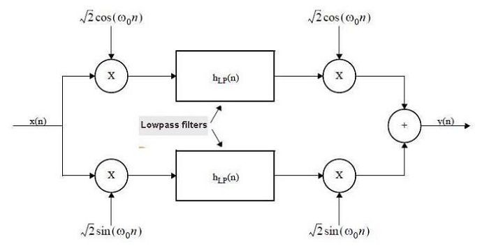
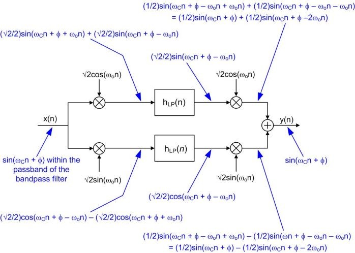
Fig 1.    The filter has complex down-conversion to baseband followed by filtering then up-conversion.  See Appendix A for a more detailed view of signal data within the filter.

THEORY OF OPERATION

Take a look at the filter block diagram above (Figure 1), which is taken from a filter design document by Momentum Data Systems[1].

This document gives the formula for the bandpass filter of Figure 1 as follows :

y₀(ω) = (h(ω - ω₀) + h(ω + ω₀)) x₀(ω)

The input signal, x(n), is processed as a vector of samples (eg from a '.wav' file), which are complex down-converted to baseband by two multipliers. Sine and cosine waveforms at the filter center frequency have the same sample length as the input signal vector. They are multiplied by the input to give baseband signals to each of the lowpass filters.

The two lowpass filters are identical, and use the MIFIR (Matrix IFIR) configuration which was described in my previous blog. The cut-off frequency of both filters is equal to half that of the desired bandpass width. After filtering, the complex up-conversion process converts the signal back to the input frequency.  For more interesting information on complex (quadrature) techniques, I can recommended this blog.
Note that the sample rate remains constant throughout the filter. In other words, there is no downsampling and upsampling.
There are just five parameters to be set which are as follows:

Bandpass width,  transition region width,  center frequency,  taps1,  taps2.

The taps1 parameter determines the stopband attenuation and passband ripple, while the taps2 value controls suppression of spurious products in the stopband.  The taps1 value will normally be greater than five times that of taps2.  It is suggested that the values given in the example (taps1 = 89 and taps2 = 15) are used as a starting point, and small changes made to tailor the response.

CODE WITH EXAMPLE PARAMETERS

The code listing below features parameters for a bandpass filter with a passband width of 10 Hz and ripple of less than 1 dB. The transition region width is 13 Hz wide with greater than 60 dB attenuation outside this range.
So what’s all this code doing ?   Well, despite the rather long software listing below, once the filter coefficients are calculated from the ‘remez’ routines, the filter process requires just fourteen lines.  Most of the remainder is to show plots of the results.
Note that there are a few combinations of input parameters for which the ‘remez’ algorithm may not converge.  This can be corrected by small changes to either the input parameters, or the value of parameters taps1 and/or taps2.
The software runs without modification in Octave version 5.1 or Matlab R2016b.
Figure 2 shows the filter response obtained with default values for taps1 and taps2.  View more detailed plots, including an FFT of the chirp output signal, by running the code.

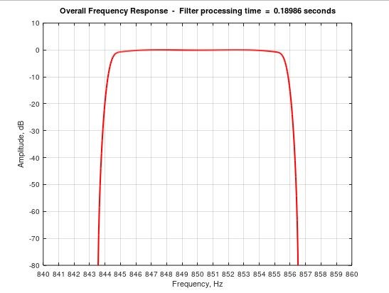
Fig 2.  The filter response here uses the default design values of 48 kHz sample rate, 850 Hz center frequency, 10 Hz bandwidth, 13 Hz transition region, with values for taps1 and taps2 of 89 and 15 respectively.

The filter processing time is the time taken to process the input signal (eg the 5 second chirp signal in the example), between locations (A) and (H) of Figure 1.
This shows up in the Octave or Matlab command window, and at the top of each plot.
If the 'comparison_filter' variable near the top of the listing is set to 'true', then the filter processing time can be compared with that of a conventional single stage filter. The result is displayed in the Octave or Matlab command window.  Figure 3 shows the frequency response plot for the 50,000 tap single stage filter.

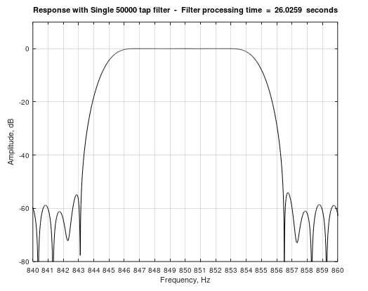
Fig 3.  The single stage 50000 tap comparison filter has a much longer processing time – compare this with Figure 2 (both run in Octave on Windows 10).

CONCLUSION

The efficient bandpass filter described has been designed for easy implementation in either Octave or Matlab. Comments and suggestions for adapting and/or improving the code are most welcome.

%
%                       FIR narrow bandpass filter
%                  ==========================

%                           Paul Lovell   June 2020

   %   This program runs in Octave 5.1 using the 'remez' function
   %   (from the Octave-Forge 'signal' package), or in Matlab.
   %   
   %   Specification for this bandpass filter example :
   %   Center frequency:               850 Hz
   %   Passband:                            10 Hz at < 1dB
   %   Transition Region:              13 Hz at > 60dB
   %   Sample rate:                         48 kHz
   %
   %   The taps in the first and second stages of the two lowpass
   %   filters can be set to any number > 3, as required. 
   %   Higher stopband attenuation, and/or a sharper transition
   %   band will require more taps.
   %   
          
%  ***********************  Input Parameters  **********************
  
   %   Set the bandpass filter input parameters as required
   %
   clear all;
   Fs = 48000;            % Set sample rate in Hz
   passband = 10;         % Set passband width Hz
   stopband = 13;         % Set stopband limit Hz
   cfr = 850;             % Set the center frequency
   taps1 = 89;            % Set taps for first stage MIFIR filter 
   taps2 = 15;            % Set taps for second stage MIFIR filter 
  
   %  Set the test signal duration as required. 
   signal_block_drn = 5;    % test signal duration in seconds
   
   comparison_filter = false;    
   %  This is used to check the relative processing duration and
   %  compare it with a window method single stage filter
  
   dt = 1/Fs;
   tw = 0:dt:signal_block_drn; 
      
   psb = passband/2;
   stb = stopband/2;
   
   %  Test Chirp Signal input to the filter
   %  Replace this with your own input signal as required
   
   chfmin = 0; chfmax = Fs/2;
   sig = chirp(tw,chfmin,signal_block_drn,chfmax)';
   siglen = length(sig);
        
%  *****************  Down/up-conversion oscillators  *************  
  
   sinosc = sqrt(2) * sin(2*pi*cfr*tw)';
   cososc = sqrt(2) * cos(2*pi*cfr*tw)';
      
%  *******  Calculate filter passband and stopband parameters  *******
  
   m2 = round(Fs/(6 * (psb+stb)));      % interpolation for filter 2
   m1 = 3 * m2;                         % interpolation for filter 1
      
   pf = double(2 * psb * m1)/Fs; 
   sf = 1-pf;
        
   f = [0 pf sf 1];                     % MIFIR-1 design parameters
   b1 = remez(taps1-1, f, [1 1 0 0], [1 1]); 
      
   f = [0 0.199 0.451 1];               % MIFIR-2 design parameters
   b2 = remez(taps2-1, f, [1 1 0 0], [1 8]);
   
   scale = 1.02/sqrt(m1^2*m2);          % scaling factor 
   b1 = b1*scale; b2 = b2*scale;        % scale coefficients 
   
   bsig = zeros(length(sig),2);
          
%  *******************  Signal down-conversion  ****************

   tstart = tic; 
     
   bsig(:,1) = sig .* cososc;
   bsig(:,2) = sig .* sinosc;
  
   % *********  Five stage baseband lowpass filters ********
   %
 for ix = 1:2 
       
   sig2 = [bsig(:,ix); zeros(mod(-siglen,m1),1)]; % zero padding
   sg1 = filter(b1,1,reshape(sig2,m1,[])')';      % 1st stage (MIFIR)
   sg2 = filter(b2,1,reshape(sg1,m2,[])')';       % 2nd stage (MIFIR)
   
   sg3 = reshape(sg2,[],1); 
      
   sg3 = cumsum(sg3-[zeros(m1,1); sg3(1:end-m1)]); % 3rd stage RRS
   sg3 = cumsum(sg3-[zeros(m1,1); sg3(1:end-m1)]); % 4th stage RRS
       
   sg4(:,ix) =  cumsum(sg3-[zeros(m2,1);sg3(1:end-m2)]);
                                                   % 5th stage RRS
 end 
 
%  *******************  Signal up-conversion  **************** 
 
   sg5 = sg4(1:siglen,1) .* cososc; 
   sg6 = sg4(1:siglen,2) .* sinosc;      
   sig_out = sg5 + sg6; 
   
   timefilt =  num2str(toc(tstart)); 
   disp(['Processing with dual 5 stage filter  ' ...
   timefilt '  seconds']);
       

%  ******** FFT routines for frequency response plots **********  
   
   FFTsize = 2^(17+floor(log10(Fs/psb))); % Adjust FFT to passband
   fp = Fs/1000; 
   b1 = b1/scale; b2 = b2/scale;         % Rescale to display MIFIRs
   b3 = ones(m1,1)*scale; b4 = b3;       % Rescale to display RRS
   b5 = ones(m2,1);
   [H1,F1] = freqz(b1,1,FFTsize,fp);     % Spectrum of prototype filter
   b1u = upsample(b1,m1);
   [H1u,F1] = freqz(b1u,1,FFTsize,fp);   % Spectrum of matrix filter 1
   
   [H2,F2] = freqz(b2,1,FFTsize,fp);     % Spectrum of prototype filter
   b2u = upsample(b2,m2); 
   [H2u,F2] = freqz(b2u,1,FFTsize,fp);    % Spectrum of matrix filter 2
   
   [H3,F3] = freqz(b3,1,FFTsize,fp);     % Spectrum of filter 3 (RRS)
   [H4,F4] = freqz(b4,1,FFTsize,fp);     % Spectrum of filter 4 (RRS)
   [H5,F5] = freqz(b5,1,FFTsize,fp);     % Spectrum of filter 5 (RRS)
   [H6,F6] = freqz(sig_out,1,FFTsize,fp); 
   
   H = H1u.*H2u.*H3.*H4.*H5; % The overall filter frequency response
   
%  ********************  Graphic Display Function ****************** 
   
   % amplitude vs frequency plots to show passband and stopband
   % x-axis may be changed with a different plot width parameter
   % this is the first of the four parameters for the plots below
  
   filter_plot(1,:) =  [2 10 10 -80] ;
   filter_plot(2,:) =  [20 10 10 -80] ;
   filter_plot(3,:) =  [2 0.5 0.2 -2] ;
   filter_plot(4,:) =  [85 10 10 -80] ;
    
   H = vertcat(flipud(abs(H)),abs(H));    % Format the data
   H = H(1:2:length(H)); 
 
   for fig_num = 1:4
   
     figure(fig_num);
     
     plot(20*log10(H),'-r', 'linewidth', 2);
     % Calculate axes based on FFT size 
     pg = psb * filter_plot(fig_num,1);
     dmax = (FFTsize/2) + ((FFTsize * pg)/Fs);
     dmin = (FFTsize/2) - ((FFTsize * pg)/Fs);
     if cfr<pg 
      dmin = dmin + ((dmax-dmin)*(pg-(cfr/2))/(pg*2)); 
      cp = 0; cr = Fs/2; cq = cr/20;
     else 
      cp = cfr-pg; cr = cfr+pg; cq = pg/10;       
     end;
     amax = filter_plot(fig_num,2);
     intv = filter_plot(fig_num,3);
     amin = filter_plot(fig_num,4);
     axis([dmin,dmax,amin,amax]); grid on; 
     xlabel('Frequency, Hz'); ylabel('Amplitude, dB');
   
     set (gca, 'xtick',[dmin:(dmax-dmin)/20:dmax]);
     set (gca, 'xticklabel',[cp:cq:cr]); 
     set (gca, 'ytick',[amin:intv:amax]);
     set (gca, 'yticklabel', [amin:intv:amax]);  
     
     title_str =(['Overall Frequency Response  -  ', ...
     'Filter processing time  =  ',timefilt,' seconds']); 
     title(title_str);
   
  end
  
    figure(5);               %  FFT plot of filter output signal
  
     plot(20*log10(abs(H6)/sqrt(Fs*2)),'-r', 'linewidth', 2);
    
     dmax = 1275 * FFTsize * 2/Fs;        % Calculate axes based on FFT size 
     dmin = dmax/3; amax = 10; intv = 10; amin = -80;
     smax = 1275; smin = 425;
     axis([dmin,dmax,amin,amax]); grid on; 
     xlabel('Frequency, Hz'); ylabel('Amplitude, dB');
    
     set (gca, 'xtick',[dmin:(dmax-dmin)/20:dmax]);
     set (gca, 'xticklabel',[smin:(smax-smin)/20:smax]); 
     set (gca, 'ytick',[amin:intv:amax]);
     set (gca, 'yticklabel', [amin:intv:amax]);  
     
     title_str =(['FFT of filter output sequence -  ', ...
     'Filter processing time  =  ',timefilt,' seconds']); 
     title(title_str);
        
   if comparison_filter
      % Compares response with single stage filter (Hamming window)
      % for default parameters.
     
     b_ref = fir1(50000,[0.035208 0.035625]);
     [Href,Fref] = freqz(b_ref,1,FFTsize,Fs); % Frequency response 
     figure(6); plot(Fref,20*log10(abs(Href)),'-k'); 
     axis([840,860,-80,10]); grid on; xlabel('Frequency, Hz');
     ylabel('Amplitude, dB');
     set (gca, 'xtick',[840:1:860]);
     set (gca, 'xticklabel',[840:1:860]); 
   
     ref = tic;
     ref_filter_out = filter(b_ref,1,sig);
     timeref = num2str(toc(ref));
     t_str = ([' Single 50000 tap filter  -  ', ...
      'Filter processing time  =  ',timeref,'  seconds']);
     disp([char(10),'Processing with ',t_str,char(10)]); 
     title(strcat('Response with ',t_str));
             
   end   
    
%  ******************************************************************
%
%  This software is provided "AS IS", without warranty. The author 
%  shall not be liable for any claim, damages or other liability
%  arising from, or in connection with this software.

APPENDIX  A

REFERENCES  AND  ACKNOWLEDGEMENTS

My thanks to Richard (Rick) Lyons for assistance with providing the data in Appendix A, and also with Matlab testing.

 [1] Momentum Data Systems, http://www.mds.com/wp-content/uploads/2014/05/multirate_article.pdf, Page 8.

Sign in