How Discrete Signal Interpolation Improves D/A Conversion

• Tips and Tricks

Earlier this year, for the Linear Audio magazine, published in the Netherlands whose subscribers are technically-skilled hi-fi audio enthusiasts, I wrote an article on the fundamentals of interpolation as it's used to improve the performance of analog-to-digital conversion. Perhaps that article will be of some value to the subscribers of dsprelated.com. Here's what I wrote:

We encounter the process of digital-to-analog conversion every day—in telephone calls (land lines and cell phones), telephone answering machines, CD & DVD players, iPhones, digital television, MP3 players, digital radio, and even talking greeting cards. This material is a brief tutorial on how sample rate conversion improves the quality of digital-to-analog conversion.

Ideal Digital-to-Analog Conversion
Have a look at the system shown in Figure 1(a). There we show a hardware depiction of a digital-to-analog converter (DAC)—a hardware device having multiple input pins that accept multibit binary words. In that figure the variable x(n) represents a sequence of binary words showing their individual binary bits from the least significant bit (LSB) to the most significant bit (MSB). In Figure 1(b) we show a hypothetical time-domain sequence of x(n) amplitude values, which we'll call "samples", where each sample is represented as a single black dot. We refer to the x(n) signal as a discrete, or "digital", sequence. The variable n is referred to as the "time-domain index" of the discrete x(n) input signal. Critical to its operation, the DAC accepts a periodic-in-time, pulse-like, signal shown as f_clk in Figure 1(a). The repetition rate, the frequency, of the f_clk signal is the reciprocal of the time period between individual x(n) samples. The f_clk signal, synchronized with the binary x(n) input sequence, triggers the DAC to 'clock in' the bits of the current x(n) sample.

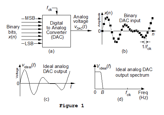
Finally, the DAC has a single output pin upon which is riding an analog (what the digital signal processing experts call "continuous") voltage that we'll call v_DAC(t). The variable t in v_DAC(t) represents time measured in seconds. Given the x(n) input sequence shown in Figure 1(b), we wish to generate the analog v_ideal(t) signal shown in Figure 1(c) whose frequency-domain spectrum is depicted in Figure 1(d). In our frequency plots we only show the positive-frequency axis because we assume all signals are real-valued and all spectra are symmetrical and centered at zero Hz.

The Nyquist Criterion
In this discussion, if the highest-frequency spectral component of x(n), and therefore v_ideal(t), is B Hz, we're assuming that the f_clk sample rate is greater than 2B Hz. That condition is the famous Nyquist criterion stipulating the periodic sampling condition required for error-free sampling (analog-to-digital conversion) of analog signals. As a historical note, the notion of periodic sampling was studied by various engineers, scientists, and mathematicians such as the Russian V. Kotelnikov, the Swedish-born H. Nyquist, the Scottish E. Whittaker, and the Japanese I. Someya [1]. But it was the American mathematician Claude Shannon, acknowledging the work of others, that mathematically formalized the concept of periodic sampling as we know it today, named it in honor of the great American electrical engineer Harry Nyquist, and brought it to the broad attention of the world's communications engineers [2]. That was in 1948—the birth year of the transistor, marshmallows, and this author.

OK, back to Figure 1. Unfortunately, commercially-available DACs will not produce our desired v_ideal(t) output voltage based on the x(n) input sequence. So, given that apparently bad news, let's now think about some hypothetical, and actual, DAC output signals and their spectra.

Some Hypothetical DAC Output Signals
If we could build a DAC whose output voltage was a periodic series of super-narrow (widths measured in picoseconds) analog pulses as shown in Figure 2(a), whose amplitudes are equal the to amplitudes of x(n), the spectrum of such analog pulses would be the repetitive pattern shown in Figure 2(b).

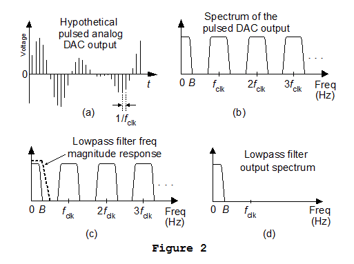
Figure 2 illustrates one of the relationships between the time- and frequency-domain representations of a signal: if a time signal has periodic amplitude variations, such as the periodically-spaced pulses in Figure 2(a), its spectrum will be periodic. If our time signal's super-narrow pulses are separated by 1/f_clk seconds, the repetitive spectral energy will be separated by f_clk Hz as shown in Figure 2(b).

Now if we passed the analog pulsed signal in Figure 2(a) through an analog lowpass filter, whose frequency magnitude response is shown by the dashed lines in Figure 2(c), we'd produce our desired Figure 1(c) v_ideal(t) signal having the spectrum shown in Figure 2(d). As straightforward as all of this seems to be, as it turns out, the electronics needed to generate the super-narrow Figure 2(a) pulses is prohibitively expensive, on the order of the cost of a new Harley Davidson Sportster motorcycle. Far too costly to include in any telephone, music, or television product. Thankfully, DAC manufacturers have a far more affordable way of generating our desired v_ideal(t) signal.

Thinking again about Figure 1, we can view the discrete x(n) sample values in Figure 1(b) as being amplitude samples of our desired v_ideal(t) analog signal in Figure 1(c). What we want is an interpolated version of x(n). But not merely two or four or ten new samples between each original x(n) sample, we seek an infinite number of samples between each original x(n) sample. We want so many new samples that our interpolated signal is continuous (analog). It's not traditional interpolation we desire, we wish to perform interpolation on steroids. This notion of interpolation is not unusual. Some signal processing experts refer to the DAC process itself as interpolation [3].

Thinking about our idea of interpolation, it would nice if we could build a DAC whose output voltage was that shown by the solid curve in Figure 3(a). As it turns out, that solid curve in Figure 3(a) is not a curve at all—it's a series of straight lines connecting the x(n) sample values shown by the shaded dots.

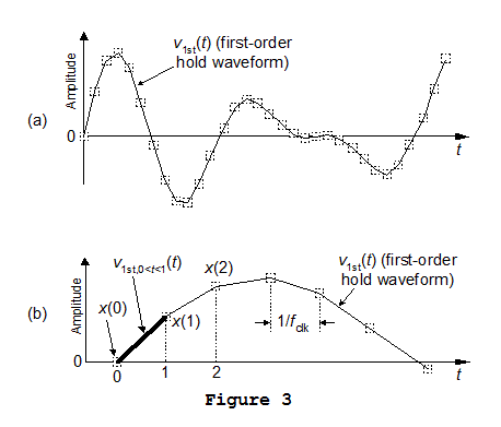
Let's zoom in and think about the first bold-line segment of that curve as shown in Figure 3(b). To generate the voltage segment between the x(0) and x(1) amplitude values we'd have to electronically evaluate the following expression:

      v_1st(t) = x(0) + [x(1) – x(0)]t,     for 0 ≤ t < 1.       (1)

Equation (1) is a first-order (first-order in terms of t) polynomial, and that's why the v_1st(t) curve comprising the connected straight lines is called a "first-order hold" waveform. (The process of generating the v_1st(t) waveform, based on the x(n) samples, is called "curve fitting" by signal processing folk. As with the hypothetical voltage in Figure 2(a), the electronic components needed to generate v_1st(t) would be prohibitively expensive for our DAC applications. Let's now review the less-expensive method for generating our desired v_ideal(t) signal developed by commercial DAC designers.

Actual DAC Output Signals
Given the discrete x(n) input sequence shown in Figure 1(b), a commercially-available DAC output voltage will be the analog v_DAC(t) signal shown in Figure 4(a). To generate the v_DAC(t) voltage segment between the x(0) and x(1) amplitude values we need merely implement the following expression:

       v_DAC(t) = x(0),     for 0 ≤ t < 1        (2)

which is not a function of time t. Likewise, between the x(1) and x(2) amplitude values the v_DAC(t) voltage is merely an implementation of:

       v_DAC(t) = x(1),     for 1 ≤ t < 2.        (3)

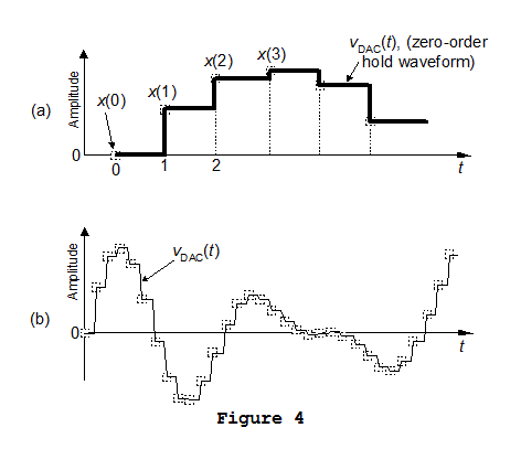
Equations (2) and (3) are referred to as "zero-order polynomials" because we could write Eq. (3), for example, as

       v_DAC(t) = x(1)t⁰,     for 1 ≤ t < 2.        (4)

Notice that the power of variable t in Eq. (4) is zero. The v_DAC(t) signal is commonly called a "zero-order hold" waveform [3]. Zooming out from Figure 4(a) we see a longer-time interval of the v_DAC(t) signal in Figure 4(b).

Now that we know the zero-order hold nature of DAC analog outputs, let's determine the spectral content of such an analog voltage. To do so, we return to the hypothetical analog pulsed DAC output that we considered in Figure 2. We repeat that pulsed signal, and its repetitive spectrum, in Figures 5(a) and 5(b). We can think of our DAC's 'stairstep' v_DAC(t) output signal as the convolution of the Figure 5(a) pulses with a rectangular, unity-amplitude, interpolation function shown in Figure 5(c) having the sin(x)/x spectrum given in Figure 5(d). Because convolution in the time domain is equivalent to multiplication in the frequency domain, the Figure 5(f) solid-curve spectrum of v_DAC(t) is the product of the Figure 5(b) and Figure 5(d) spectra.

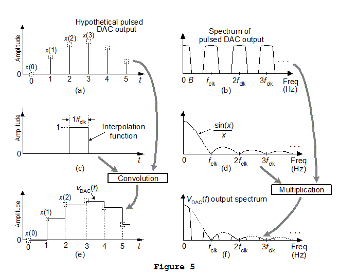
So there you have it—the spectrum of a DAC's v_DAC(t) output is the repetitive, decreasing-magnitude, spectrum given in Figure 5(f).

Post-DAC Analog Filtering
Our final task to achieve our ideal Figure 1(c) v_ideal(t) voltage, whose spectrum is in Figure 1(d), is to pass the v_DAC(t) output signal through an analog lowpass filter as shown in Figure 6(a). The lowpass filter's mandatory frequency magnitude response is shown by the dashed lines in Figure 6(b). The spectrum of our resultant v_out(t) is given in Figure 6(c), and the v_out(t) voltage, in Figure 6(d), is quite similar to our desired v_ideal(t) analog signal in Figure 1(c).

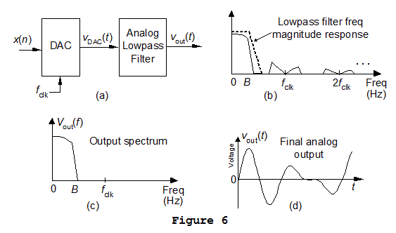
OK, there are two things we must consider regarding the DAC/filtering system in Figure 6(a). First, the DAC's non-flat Figure 5(d) sin(x)/x magnitude envelope attenuates the higher frequency spectral components in our original x(n) signal. That is, the drooping nature of a DAC's inherent sin(x)/x frequency characteristic, shown in Figure 7(a), attenuates our original signal in the vicinity of B Hz.

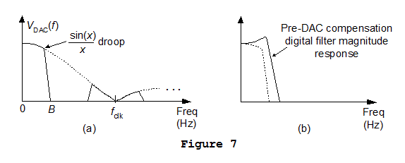
In some DAC applications, if the frequency B Hz is small relative to the f_clk frequency, perhaps we could simply ignore the sin(x)/x amplitude droop. However if the sin(x)/x droop cannot, for some reason, be tolerated, then specialized 'DAC-compensation' digital filtering must be performed in the processing steps prior to applying the x(n) sequence to the DAC. That is, our signal of interest may need to be applied to a pre-DAC compensation digital filter such as the solid curve in Figure 7(b) where the high-frequency signal components in the vicinity of B Hz are amplified. That amplification would then be canceled by the sin(x)/x droop behavior of our DAC.

The second issue for us to consider regarding the DAC/filtering system in Figure 6(a) is the complexity of the analog lowpass filter. An analog filter having a frequency magnitude response as shown by the dashed lines in Figure 6(b), with such a narrow transition region from the end of its passband to the beginning of its stopband, may be difficult to design. Such a filter may have several active electronic components and be expensive. In addition to the cost issue, analog lowpass filters have the additional problem of exhibiting nonlinear phase responses in the neighborhood of their cutoff frequency at B Hz. Fortunately, a multirate digital signal processing operation is available that can reduce both the complexity (cost) and nonlinear phase problems associated with analog lowpass filters used in DAC applications.

Digital Interpolation to the Rescue
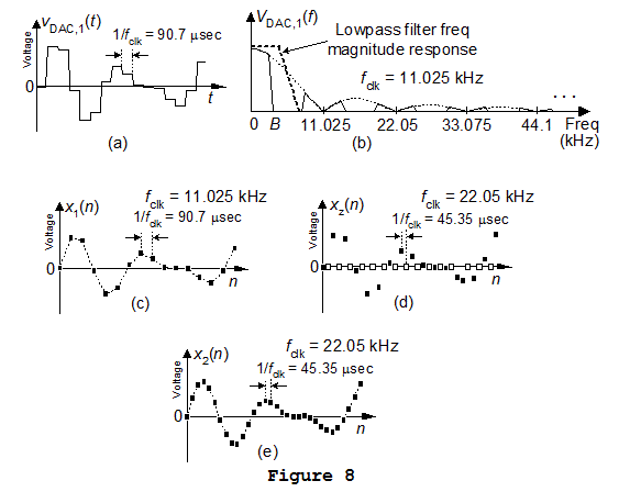
We can drastically simplify our analog lowpass filter design complexity by increasing our x(n) signal's f_clk sample rate which is our DAC's f_clk clock frequency. That is, we will interpolate our original x(n) signal. To explain this notion of interpolation, consider the v_DAC,1(t) analog DAC output signal in Figure 8(a). Assuming that the DAC's f_clk clock rate is 11.025 kHz, the spectrum of the DAC's output signal is the solid v_DAC,1(f) curve in Figure 8(b). At this 11.025 kHz clock rate the analog lowpass filter's frequency magnitude response will be the bold dashed curve in Figure 8(b). We show the DAC's x₁(n) input discrete sequence, whose sample rate is 11.025 kHz, in Figure 8(c).

We implement a 'digital interpolation-by-two' process as follows: First, prior to any DAC processing, we insert a zero-valued sample in between each of the x₁(n) samples to generate the x_z(n) sequence shown in Figure 8(d). (The inserted samples are shown by white dots in Figure 8(d). The full time durations of the x₁(n) and x_z(n) sequences, from their first to their last samples, measured in seconds, are identical.) Next we merely pass the x_z(n) sequence through a digital lowpass filter whose cutoff frequency is slightly greater than B Hz. That filter's output, then, will be the 22.05 kHz sample rate interpolated x₂(n) sequence shown in Figure 8(e).

So, the most simple form of digital interpolation is a two-step process: zero-valued sample insertion followed by digital lowpass filtering. A more thorough discussion of digital interpolation can be found in chapter 10 of reference [4].

Applying the interpolated x₂(n) discrete sequence to our DAC generates the v_DAC,2(t) voltage shown in Figure 9(a). The neat part here is that the spectrum of v_DAC,2(t) is that shown in Figure 9(b). The analog lowpass filter, whose frequency magnitude response is the bold dashed curve in Figure 9(b), has a much more gradual (wider) transition region from the end of its passband to the beginning of its stopband. This means the v_DAC,2(f) lowpass filter is simpler and much less expensive than the v_DAC,1(f) lowpass filter.

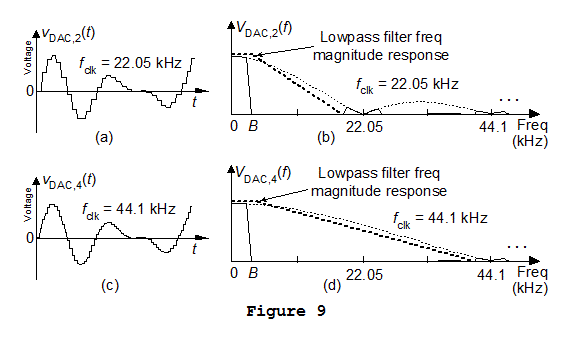
There are two additional advantages of our factor of two interpolation. First the undesirable spectral noise centered at 22.05 kHz in Figure 9(b) is smaller in magnitude than the spectral noise centered at 11.025 kHz in Figure 8(b). Second, the digital lowpass filter used in our digital interpolation process can be designed to implement the desirable pre-DAC compensation in Figure 7(b).

We could go one step further and interpolate sequence x₂(n) by another factor of two to generate a discrete x₄(n) sequence having a 44.1 kHz sample rate. Applying that x₄(n) sequence to our DAC will generate the v_DAC,4(t) voltage in Figure 9(c) whose spectrum is given in Figure 9(d). The analog lowpass needed for the v_DAC,4(t) signal, the bold dashed curve in Figure 9(d), can be quite simple now, perhaps merely a few resistors and capacitors.

Concluding Remarks
We started this presentation with a discussion of ideal digital-to-analog conversion. Realizing that we cannot perform such an ideal conversion, we considered a few hypothetical digital-to-analog conversion scenarios to help use understand the behavior of commercially-available digital-to-analog converters (DACs). We see that, due to real-world DAC imperfections, analog lowpass filters are needed for proper digital-to-analog conversion. Finally, we showed how digital signal interpolation can be used to drastically reduce the complexity and cost of the analog lowpass filters. (Remember, if we can reduce the cost of our analog filter by 50 cents, and we sell 6 million units, we've saved three million dollars!) The digital interpolation scheme used to reduce analog circuit complexity is a classic example of how digital signal processing can be used to build lower-cost, more reliable, systems. In addition, such digital interpolation has the benefit of reducing the sin(x)/x droop effects of our DAC, and that improves the quality of the final analog lowpass filter's v_out(t) signal.

References
[1] Luke, H. “The Origins of the Sampling Theorem,” IEEE Communications Magazine, April 1999, pp. 106–109.

[2] Shannon, C. “A Mathematical Theory of Communication,” Bell Sys. Tech. Journal, Vol. 27, 1948, pp. 379–423, 623–656.

[3] Prandoni, P. and Vetterli, M., "Signal Processing For Communications", EPFL Press, Lausanne, Switzerland, 2008, pp. 240-247.

[4] Lyons, R., "Understanding Digital Signal Processing" 3rd Ed., Prentice Hall Publishing, Upper Saddle River, NJ, 2010, pp. 507-588.

Sign in