Simultaneously Computing a Forward FFT and an Inverse FFT Using a Single FFT

• Tips and Tricks

Most of us are familiar with the processes of using a single N-point complex FFT to: (1) perform a 2N-point FFT on real data, and (2) perform two independent N-point FFTs on real data [1–5]. In case it's of interest to someone out there, this blog gives the algorithm for simultaneously computing a forward FFT and an inverse FFT using a single radix-2 FFT.

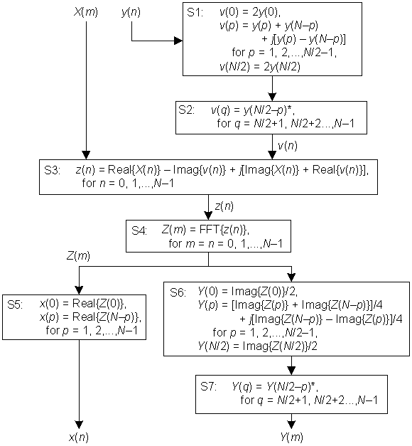
Our algorithm is depicted by the seven steps, S1 through S7, shown in Figure 1. In that figure, we compute the x(n) inverse FFT of the N-point frequency-domain conjugate symmetric input sequence X(m), as well as compute the Y(m) forward FFT of the N-point time-domain real-valued input sequence y(n) using the single complex FFT in step S4. Sample indices n and m both range from 0 to N–1 where N is an integer power of two.

At first glance Figure 1 looks more complicated than it actually is, and here's why:

• Steps S1 and S2 create a complex sequence that we call v(n).
• Step S1 generates the first N/2+1 samples of v(n) based on the real-valued input sequence y(n).
• Step S2 extends v(n) to a length of N samples and forces v(n) to be conjugate symmetric. The '*' symbol in step S2 means conjugation.
• Step S3 combines the conjugate symmetric sequences X(m) and v(n) to create a sequence we call z(n). (Sequence z(n) is not conjugate symmetric.)
• Step S4 is the algorithm's single radix-2 FFT operation, generating complex sequence Z(m).
• Step S5 generates the desired real-valued x(n) time sequence by performing a circular reversal of the real part of Z(m). (That is, other than the first sample, the real part of Z(m) samples are reversed in order to produce x(n).)
• Steps S6 and S7 generate the desired frequency-domain Y(m) sequence.
• Step S6 generates the first N/2+1 samples of Y(m).
• Step S7 extends the sequence from step S6 to a length of N samples, and forces conjugate symmetry, to produce Y(m). The '*' symbol in step S7 means conjugation.

I didn't invent this algorithm. Figure 1 is my interpretation and implementation of the discussion in Reference [6]. The Figure 1 algorithm's computational workload is one complex N-point FFT and roughly 2N additions/subtractions.

Below is a bit of MATLAB code demonstrating the process in Figure 1.

clear all, clc
% Create test input vectors
    True_x = [1, 2, 3, 4, 5, 6, 7, 8]
    X = fft(True_x);
    y = [0.1, 0.2, 0.3, 0.4, 0.5, 0.6, 0.7, 0.8];
    True_Y = fft(y)
N = length(X);
% Create vector "v"
    v(1) = 2*y(1);       % Zero Hz sample
    for p = 2:N/2        % Create 1st half of vector "v"
        v(p) = y(p) + y(N-p+2) + j*(y(p) -y(N-p+2));
    end
    v(N/2+1) = 2*y(N/2+1);  % Fs/2 sample
    % Append conj. 2nd part of "v" vector
        v(N/2+2:N) = fliplr(conj(v(2:N/2))); 
% Create vector "z"
    z = real(X) -imag(v) + j*(imag(X) + real(v));
% Perform single FFT
    Z = fft(z); 
% Create time-domain vector "x"
    Real_Z = real(Z);
    x = [Real_Z(1), fliplr(Real_Z(2:end))]/N
% Create freq-domain vector "Y"
    Imag_Z = imag(Z);
    Y(1) = Imag_Z(1)/2; % Zero Hz sample
    for p = 2:N/2       % Create 1st half of vector "Y"
        Y(p) = (Imag_Z(p) + Imag_Z(N-p+2) + ...
            j*(Imag_Z(N-p+2) - Imag_Z(p)))/4;
    end
    Y(N/2+1) = Imag_Z(N/2+1)/2; % Fs/2 sample
    % Append conj. 2nd part of "Y" vector
        Y(N/2+2:N) = fliplr(conj(Y(2:N/2)))
% Stick a fork in me.  I'm done.

References:
[1] Lyons, R. Understanding Digital Signal Processing, 2/E, Prentice Hall, Englewood Cliffs, New Jersey, 2004, pp. 488-500.

[2] Brigham, E. The fast Fourier Transform and Its Applications, Prentice Hall, Englewood Cliffs, New Jersey, 1988.

[3] Sorenson, H. et al., "Real Valued Fast Fourier Transform Algorithms," IEEE Trans. on Acoust. Speech, and Signal Proc., Vol. ASSP 35, No. 6, June 1987.

[4] Cooley, J. et al., "The Fast Fourier Transform Algorithm: Programming Considerations In the Calculation of Sine, Cosine and Laplace Transforms," Journal Sound Vib., Vol. 12, July 1970.

[5] Burrus, C. et al., Computer-Based Exercises for Signal Processing, Prentice Hall, Englewood Cliffs, New Jersey, 1994, pp. 53.

[6] Moshe, S. and Hertz, D. "On computing DFT of real N-point vector and IDFT of DFT-transformed real N-point vector via single DFT", Signal Processing Letters, IEEE, Volume: 6, Issue: 6, June 1999, p. 141.

Sign in