


Multilayer Perceptrons and Event Classification with data from CODEC using Scilab and Weka
For my first blog, I thought I would introduce the reader to Scilab [1] and Weka [2]. In order to illustrate how they work, I will put together a script in Scilab that will sample using the microphone and CODEC on your PC and save the waveform as a CSV file. Then, we can take the CSV file and open it in Weka. Once in Weka, we have a lot of paths to consider in order to classify it. I use the term classify loosely since there are many things you can do with data sets in Weka. Your application will most likely determine how you use Weka. For this blog, I thought it would be cool to look at a Multilayer Perceptron [3], a type of Artificial Neural Network [4], in order to classify whatever I decide to record from my PC. So, if you want to follow along, go ahead and download and install Scilab and Weka.
While, I’m pretty familiar with Scilab, as you may be too, I am not an expert with Weka. I took one machine learning course while working on my Ph.D. (almost 4 years ago) and we used Weka to illustrate many different regression, classification, clustering, etc. types of machine learning algorithms one can use when presented with a data set. I was hoping to find time to look into it again. Now seems like a good time. Please chime in and give feedback. I’d like to consider this blog (and future ones) an open forum as well.
Don’t forget to check out the data set repositories at UC Irvine [5]. You can use those for examples if you don’t have a data set readily available. While we aren’t going to design a neural network CPU [6] like Skynet did in the Terminator movies, this will at least introduce to the reader to DSP tools and methods other than the traditional DSP techniques most are familiar with.
I would consider this a matched filter because I want to determine (classify) if an “event” is true (pass) or false (fail). The classifiers in my case will be just that, pass or fail (I have questions about this later). Consider someone speaking into a microphone. If they say the word “terminator”, we want a light to turn on (pass). Else, the light remains off (fail). A MLP is one method of attempting to solve this problem; although, I don’t think Pee Wee used this method to trigger the bells, whistles, and screams when someone said the secret word of the day.
Keeping it brief (since this blog isn’t an attempt to fully explore MLPs and their structure), an MLP is a type of artificial neural network. The network can be comprised of many layers, typically at least three – one input, one hidden, and one output. The inputs (input layer) are weighted and then summed at each hidden layer node. Once complete, this weighted sum is used as the input to an activation function. Then, the outputs of the activation functions are weighted and summed at the next hidden layer. This process repeats itself for however many hidden layers are used. The output layer operates the same way as the hidden layer – a weighted sum of its inputs and then applied to an activation function. While the choice of an activation function can vary, most often the sigmoid [7] is used. I really like the MLP explanation in section 5.2 of [8], [9], and [10]. Speaking of [10], here is a list of common properties of a MLP:
- No connections within a layer
- No direct connections between input and output layers
- Fully connected between layers
- Often more than 3 layers
- Number of output units need not equal number of input units
- Number of hidden units per layer can be more or less than input or output units
To help illustrate what I just said, I setup a 3 layer MLP (see figure 1) with 10 inputs (and one bias node labeled B … which I’m seeing a lot of literature pertaining to using a bias node in lieu of using thresholds … perhaps more on that later) for the input layer, 5 nodes for the hidden layer, and 1 output node. To establish the weighted values, the network goes through a training/learning period. During this time, the network is introduced to the data set of interest and the network changes the weights in order to best classify the output. It should be noted that many training parameters can be changed to help classify the data set. I believe this is where knowledge of the application is more helpful than relying on specific equations or formulas for setting values. For example, we know dealing with low-pass filters (RC, FIR, etc.) we can calculate 3 db points, ripple, etc. However, with the MLP, we are attempting to properly classify (predict) an event. In theory, once we have the weights, we can implement the MLP in code (I will do it in Scilab) and see how well the MLP predicts events.
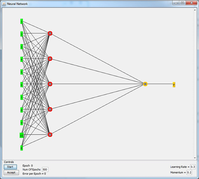
Figure 1: MLP example
This blog will look at a five MLP examples from Weka using sampled data from the microphone on my PC (with the help of Scilab). After the MLP model is generated (weights and thresholds), I’d like to implement them in Scilab in real-time, but am not sure if I will have time to do so with this blog. I think I will wait for my next blog to investigate real-time results with the models from this blog.
Ok, so you won’t find my explanation in a text book any time soon. And, if you googled or wiki’d MLP, I’m sure they did a better job explaining this. Like I said earlier, [8], [9], and [10] seem pretty good for beginners.
For my MLP, I’m starting with 10 unique events for my data set – 5 good and 5 bad. As for a good event, I simply “tap” the ThinkPad emblem on my laptop with my finger. As for bad events, I tap both sides of my computer and the three sides of my laptop screen. The other things we need to be able to bring the data set into Weka is (1) add attributes for each sample point and (2) and add a predictor/classifier for each sample set.
The attribute is just a name for each input and classifier. For the attribute labels, I create one row the same length as the number of samples and label them by each sample number (i.e. 1st sample point is attribute 1, 2nd sample point is attribute 2, etc. For example, if I were to sample one cycle of a 100 Hz waveform at 10 kHz, I would have 100 samples, and each of these samples would have an attribute label 1 through 100.). Then for the classifier, I create a 1x11 column array. The first element is the attribute which I label 99999, and then I alternate each element as 1, -1, 1, -1, etc (I actually open the CSV file after it’s complete and change 99999 to class, 1 to pass, and -1 to fail). At this point, to ensure I have enough events to train/test with, I copy the 10 events 10 times and append it to another matrix. In the end, I have 100 events – 50 good and 50 bad. Once this is all done, I save the final matrix as a CSV file.
Perhaps a good time for questions or for MLP users/experts to chime in …
Now, let’s record and use some real data. First, you’ll need to install ‘portaudio’ in order to record from the microphone on your computer. To do this, just copy and paste into the command line of Scilab:
atomsInstall('portaudio')
After it does its thing, restart Scilab and it will be (should be) ready to use. Don’t forget to check out the other ‘instrument controls’ offered by Scilab.
I’ve made a script (see attached code, CollectEvents.sce) that: records 10 events (each lasting 1 second) with a sample rate of 10 kHz, creates a matrix of 100 events and their respective attributes, and then saves it as a CSV. Once I have the CSV, I can open it in Weka. As for the 10 recorded events, every other one will be a “true” event. After the data is sampled, I save 500 of the samples containing the bulk of the capture – find the peak of the “tap” and use its index as an offset (see the code). I’m not getting into the details concerning the response/bandwidth of the microphone and sound card specifications/limitations either. I just tap, record, and save. I may need to bump up the sample rate, which will mean I’ll have to deal with more samples (and more weights).
So now we have our CSV file. One thing I do is open the CSV file and change the attribute for the classifier (99999) to class, 1 to pass, and -1 to fail. After that, open Weka and click the Explorer button. A new window will open. Once it opens, click open file and choose the CSV file from our Scilab program. Upon opening it, you are presented with some basic preprocessing options. I’m not going to do any preprocessing and just use Weka to generate the weights and thresholds I need to build a multilayer perceptron. Next to the preprocess tab you’ll see multiple tabs that can be used to classify, cluster, etc., a data set. For the purpose of this blog, click on the classify tab.
At this point, I began asking, is my data linearly separable (I mean, don’t we all ask that question when presented with a data set)? More importantly, how do I/can I map it in a way that is linearly separable? At this point, I know that one perceptron is good for classifying data that is linearly separable. If it’s not, I need more layers and perceptrons. I will use the other tabs in Weka for my next blog when I implement these models in real-time.
Under classifier, click the Choose button and select: WEKA -> CLASSIFIERS -> FUNCTIONS -> MultilayerPerceptron. Underneath, there are additional options to choose. Right-click the MultilayerPerceptron field next to the Choose button. Select show properties. At this point, I have no idea how many hidden layers are a good choice, a good learning rate, epoch time, or most of the other parameters. I’m going to start with 3 models and change the hidden layers, learning rate, and training time. Below is a table outlining the parameters to use for each:
| Parameter | Model 1 | Model 2 | Model 3 | Model 4 | Model 5 |
| GUI |
FALSE | FALSE | FALSE | FALSE | FALSE |
| autoBuild | TRUE | TRUE | TRUE | TRUE | TRUE |
| debug | FALSE | FALSE | FALSE | FALSE | FALSE |
| decay | FALSE | FALSE | FALSE | FALSE | FALSE |
| hiddenLayers | 1 | 5 | 20 | 50 | 50,2 |
| learningRate | 0.005 | 0.001 | 0.01 | 0.001 | 0.001 |
| momentum | 0.5 | 0.2 | 0.5 | 0.2 | 0.2 |
| nominalToBinaryFilter | TRUE | TRUE | TRUE | TRUE | TRUE |
| normalizeAttributes | FALSE | FALSE | FALSE | FALSE | FALSE |
| normalizeNumericClass | FALSE | FALSE | FALSE | FALSE | FALSE |
| reset | TRUE | TRUE | TRUE | TRUE | TRUE |
| seed | 0 | 0 | 0 | 0 | 0 |
| trainingTime | 100 | 1000 | 250 | 500 | 1000 |
| validationSetSize | 0 | 0 | 0 | 0 | 0 |
| validationThreshold | 20 | 20 | 20 | 20 | 20 |
One thing to note, the hidden layers parameter is comma separated where the first item is the number of nodes in the first hidden layer, the second item is the number of nodes in the 2nd hidden layer, and so on – it’s not the total number of hidden layers. Once the parameters are set, click OK.
For our case, set cross validation folds to 10. This basically splits the data sets from the file into 10 sets of 2 groups. One group is used for training and the other is used for testing. Each iteration (up to 10), a classifier is identified from the training set and then tested against with the test set. So, in the end, 10 classifiers will be identified and then each performance will be averaged. The final result showing how well classified the data is/can be.
At this point, we’re ready to run the cross validation and eventually get our result and weights. First, make sure your class is selected and then hit the start button. The Weka bird in the bottom right will start moving around and you’ll see the status change for each built model in the lower left. When finished, the status changes to OK and the Weka bird stops moving. You’ll also see a lot of numbers populate the middle screen of the window.
Repeat this while changing the parameters of the MLP until your results look good. I can get my results favorable with just 1 hidden node. But, isn’t this just one perceptron? And, does that mean my data is linearly separable? Well, I look into this some more for my next blog. I also want to implement one of these models in real-time using Scilab. You can see my results from my five models below (figures 2 – 6). Each figure shows results with its respective MLP parameters.
I hope you enjoyed reading. I welcome comments and feedback. For the most part, this was intended to present Scilab and Weka to the reader and introduce newer methods for “filtering” data, by classification. I look forward to continuing this blog and investigating these results further.
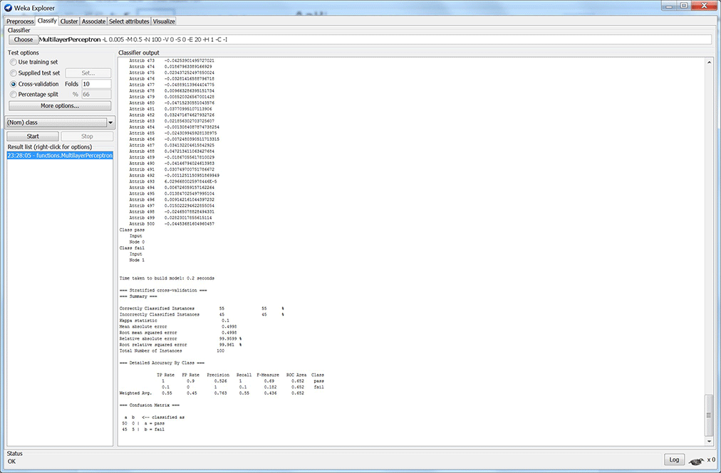
Figure 2: Model 1 results
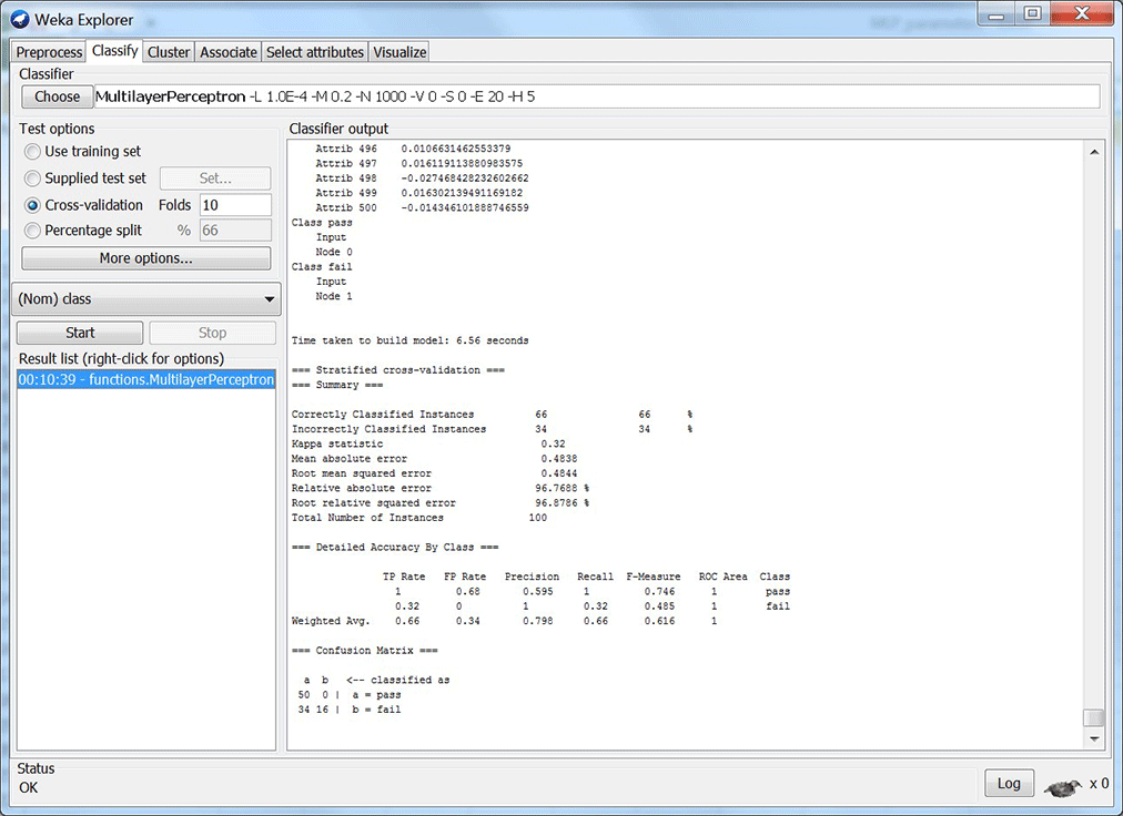
Figure 3: Model 2 results
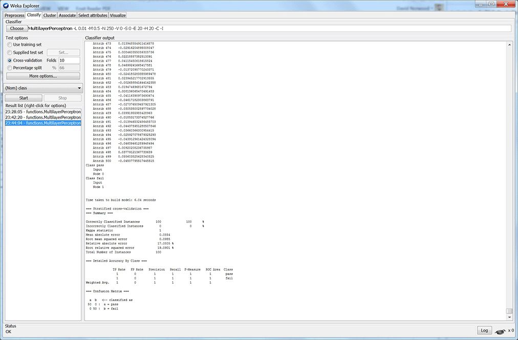
Figure 4: Model 3 results
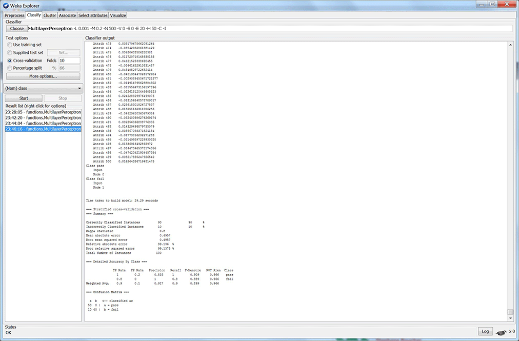
Figure 5: Model 4 results
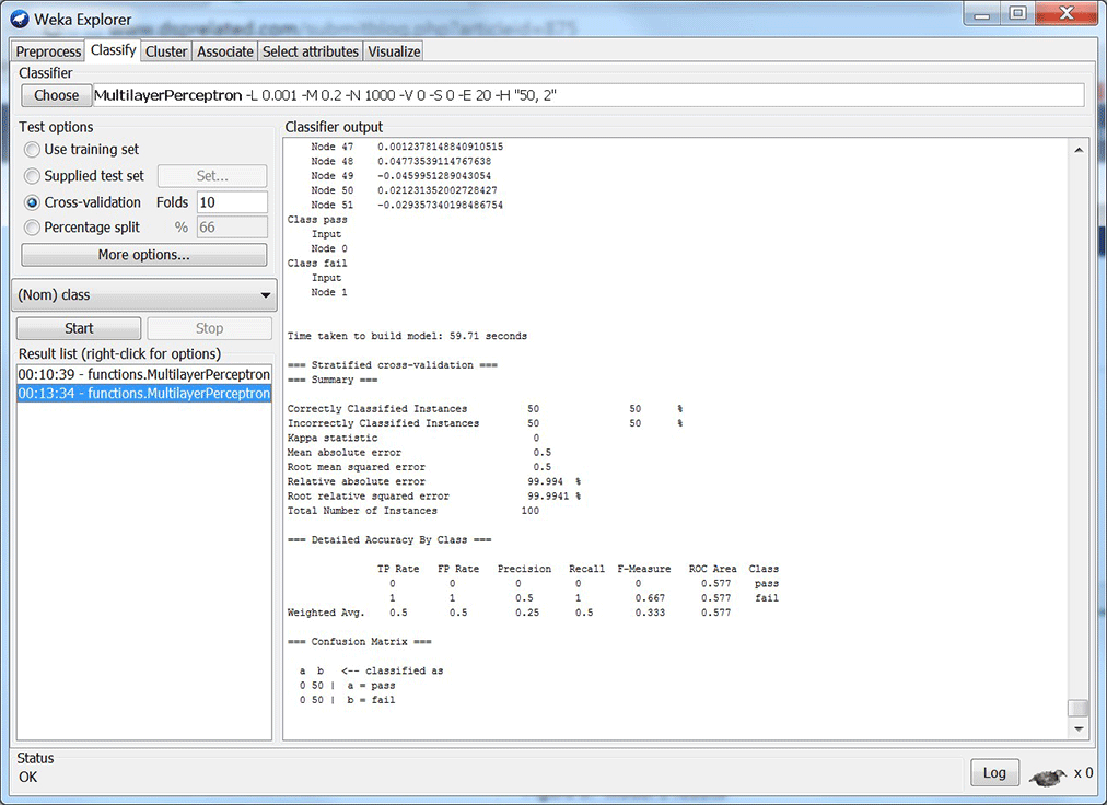
Figure 6: Model 5 results
REFERNCES:
[2] http://www.cs.waikato.ac.nz/ml/weka/
[3] https://en.wikipedia.org/wiki/Multilayer_perceptron
[4] https://en.wikipedia.org/wiki/Artificial_neural_network
[5] https://archive.ics.uci.edu/ml/datasets.html
[6] http://terminator.wikia.com/wiki/Neural_Net_CPU
[7] https://en.wikipedia.org/wiki/Sigmoid_function
[9] http://www.dspguide.com/ch26/2.htm
[10] http://www.utc.edu/center-information-security-assurance/course-listing/b2.2.mlp.ppt
- Comments
- Write a Comment Select to add a comment
To post reply to a comment, click on the 'reply' button attached to each comment. To post a new comment (not a reply to a comment) check out the 'Write a Comment' tab at the top of the comments.
Please login (on the right) if you already have an account on this platform.
Otherwise, please use this form to register (free) an join one of the largest online community for Electrical/Embedded/DSP/FPGA/ML engineers:


