


Peak-to-average ratio analysis
Determines the peak-to-average ratio of a signal for a given target percentile
Background:
Processing of communications signals - digital, analog or radio frequency - needs to be dimensioned for the dynamics of the signal, namely its average power and the maximum instantaneous power.
For example:
- Digital filters are implemented using a limited numerical range. If the numbers grow too large, saturation results
- Exceeding the maximum instantaneous power (1 dB compression point) of a radio frequency power amplifier will cause wide-band distortion products that result in interference to other channels.
- An analog-to-digital converter will clip a signal that exceeds its input range
Especially when dealing with random signals, the magnitude of peaks is not well-defined. For example, Gaussian noise has no limit to the instantaneous magnitude, even though the probability of values beyond a couple of sigmas gets rather small.
That means, in signal processing we usually cannot rule out signal clipping with certainty.
Now engineering is all about compromises, and the unavoidable question is: how much clipping is "good enough"?
The answer depends on the application. For example, the targeted uncoded symbol error rate gives some guideline: if one sample in thousand is clipped, it is unlikely to achieve a raw bit error rate of one in a million.
Peak-to-average ratio definition
For the given signal and probability, 100 * (1-probability) percent of samples will exceed a magnitude of PAR, relative to the RMS average of the signal.
Magnitude definition
For complex-valued signals, a magnitude definition needs to be selected based on what the signal represents (it does not matter for real-valued signals).
In wireless applications, a complex-valued signal s may represent in-phase and quadrature branch of a radio frequency carrier.
Clipping in radio-frequency components, such as power amplifiers, is related to the envelope of the radio frequency signal, which is abs(s).
Set independentIQ = false.
On the other hand, in baseband processing such as digital filters, real- and imaginary part of s will be handled by independent, real-valued stages.
Here, the magnitudes of real(s) and imag(s) are relevant. Since a sample is clipped when either real- or imaginary part clip, the PAR is determined based on max(abs(real(s)), abs(imag(s))).
Set independentIQ = true.
Using the code snippet
Copy into sn_headroom.m and run sn_headroom from the command line.
The function peakToAverageRatio can be copied to a file peakToAverageRatio.m.
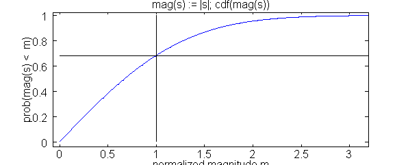
CDF plot
By default, the CDF of the magnitude (as seen by the PAR analysis) is plotted.
This part can be disabled, if not needed (if true... end)
The example shows the output from real-valued Gaussian noise with a probability target of 68.3 % (corresponding to one sigma of the normal distribution).
The algorithm looks up 68.3 % on the y axis, and reads off the normalized magnitude "1" (0 dB) on the x axis (the low percentile was chosen for plotting - practical probability targets would be >> 99 %).
% *************************************************************
% Peak-to-average analyzis of complex baseband-equivalent signal
% Markus Nentwig, 10/12/2011
% Determines the magnitude relative to the RMS average
% which is exceeded with a given (small) probability
% A typical probability value is 99.9 %, which is very loosely related
% to an uncoded bit error rate target of 0.1 %.
% *************************************************************
function sn_headroom()
    % number of samples for example signals
    n = 1e6;

    % *************************************************************
    % example: 99.9% PAR for white Gaussian noise
    % *************************************************************
    signal = 12345 * (randn(1, n) + 1i * randn(1, n));
    [PAR, PAR_dB] = peakToAverageRatio(signal, 0.999, false);
    printf('white Gaussian noise: %1.1f dB PAR at radio frequency\n', PAR_dB);
    [PAR, PAR_dB] = peakToAverageRatio(signal, 0.999, true);
    printf('white Gaussian noise: %1.1f dB PAR at baseband\n', PAR_dB);

    % *************************************************************
    % example: PAR of continuous-wave signal
    % *************************************************************
    % a quarter cycle gives the best coverage of amplitude values
    % the statistics of the remaining three quarters are identical (symmetry)
    signal = 12345 * exp(1i*2*pi*(0:n-1) / n / 4);

    % Note: peaks can be below the average, depending on the given probability
    % a possible peak-to-average ratio < 1 (< 0 dB) is a consequence of the
    % peak definition and not unphysical.
    % For a continuous-wave signal, the average value equals the peak value,
    % and PAR results slightly below 0 dB are to be expected.
    [PAR, PAR_dB] = peakToAverageRatio(signal, 0.999, false);
    printf('continuous-wave: %1.1f dB PAR at radio frequency\n', PAR_dB);
    [PAR, PAR_dB] = peakToAverageRatio(signal, 0.999, true);
    printf('continuous-wave: %1.1f dB PAR at baseband\n', PAR_dB);

    % *************************************************************
    % self test:
    % For a real-valued Gaussian random variable, the probability
    % to not exceed n sigma is
    % n = 1: 68.27 percent
    % n = 2: 95.5 percent
    % n = 3: 99.73 percent
    % see http://en.wikipedia.org/wiki/Normal_distribution
    % section "confidence intervals"
    % *************************************************************
    signal = 12345 * randn(1, n);
    [PAR, PAR_dB] = peakToAverageRatio(signal, 68.2689/100, false);
    printf('expecting %1.3f dB PAR, got %1.3f dB\n', 20*log10(1), PAR_dB);
    [PAR, PAR_dB] = peakToAverageRatio(signal, 95.44997/100, false);
    printf('expecting %1.3f dB PAR, got %1.3f dB\n', 20*log10(2), PAR_dB);
    [PAR, PAR_dB] = peakToAverageRatio(signal, 99.7300/100, false);
    printf('expecting %1.3f dB PAR, got %1.3f dB\n', 20*log10(3), PAR_dB);
end

function [PAR, PAR_dB] = peakToAverageRatio(signal, peakProbability, independentIQ)
    1;
    % force row vector
    assert(min(size(signal)) == 1, 'matrix not allowed');
    signal = signal(:) .';

    assert(peakProbability > 0);
    assert(peakProbability <= 1);

    % *************************************************************
    % determine RMS average and normalize signal to unity
    % *************************************************************
    nSamples = numel(signal);
    sAverage = sqrt(signal * signal' / nSamples);
    signal = signal / sAverage;

    % *************************************************************
    % "Peaks" in a complex-valued signal can be defined in two
    % different ways:
    % *************************************************************
    if ~independentIQ
        % *************************************************************
        % Radio-frequency definition:
        % ---------------------------
        % The baseband-equivalent signal represents the modulation on
        % a radio frequency carrier
        % The instantaneous magnitude of the modulated radio frequency
        % wave causes clipping, for example in a radio frequency
        % power amplifier.
        % The -combined- magnitude of in-phase and quadrature signal
        % (that is, real- and imaginary part) is relevant.
        % This is the default definition, when working with radio
        % frequency (or intermediate frequency) signals, as long as a
        % single, real-valued waveform is being processed.
        % *************************************************************
        sMag = abs(signal);
        t = 'mag(s) := |s|; cdf(mag(s))';
    else
        % *************************************************************
        % Baseband definition
        % -------------------
        % The baseband-equivalent signal is explicitly separated into
        % an in-phase and a quadrature branch that are processed
        % independently.
        % The -individual- magnitudes of in-phase and quadrature branch
        % cause clipping.
        % For example, the definition applies when a complex-valued
        % baseband signal is processed in a digital filter with real-
        % valued coefficients, which is implemented as two independent,
        % real-valued filters on real part and imaginary part.
        % *************************************************************
        % for each sample, use the maximum of in-phase / quadrature.
        % If both clip in the same sample, it's counted only once.
        sMag = max(abs(real(signal)), abs(imag(signal)));
        t = 'mag(s) := max(|real(s)|, |imag(s)|); cdf(mag(s))';
    end

    % *************************************************************
    % determine number of samples with magnitude below the "peak"
    % level, based on the given peak probability
    % for example: probability = 0.5 => nBelowPeakLevel = nSamples/2
    % typically, this will be a floating point number
    % *************************************************************
    nBelowPeakLevel = peakProbability * nSamples;

    % *************************************************************
    % interpolate the magnitude between the two closest samples
    % *************************************************************
    sMagSorted = sort(sMag);
    x = [0 1:nSamples nSamples+1];
    y = [0 sMagSorted sMagSorted(end)];
    magAtPeakLevel = interp1(x, y, nBelowPeakLevel, 'linear');

    % *************************************************************
    % Peak-to-average ratio
    % signal is normalized, average is 1
    % the ratio relates to the sample magnitude
    % "power" is square of magnitude => use 20*log10 for dB conversion.
    % *************************************************************
    PAR = magAtPeakLevel;
    PAR_dB = 20*log10(PAR + eps);

    % *************************************************************
    % illustrate the CDF and the result
    % *************************************************************
    if true
        figure();
        plot(y, x / max(x));
        title(t);
        xlabel('normalized magnitude m');
        ylabel('prob(mag(s) <  m)');
        line([1, 1] * magAtPeakLevel, [0, 1]);
        line([0, max(y)], [1, 1] * peakProbability);
    end
end


