


Digital model for analog filters
Modeling an analog (continuous-time) component in a digital (discrete-time) environment using a sampled impulse response.
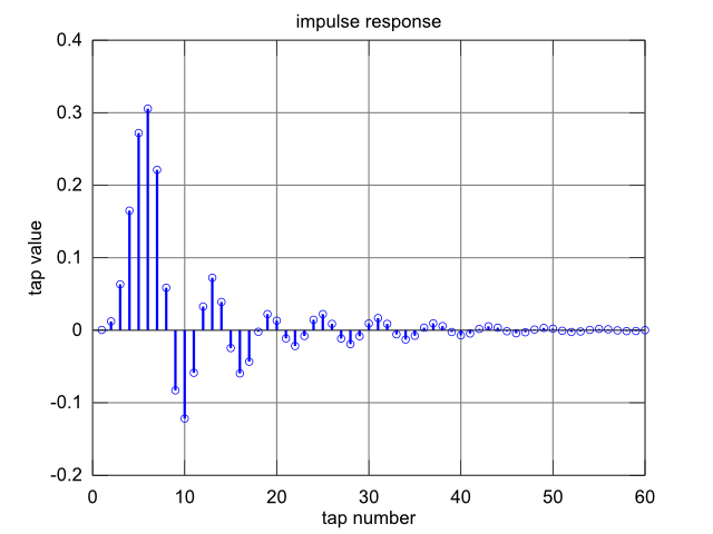
Example impulse response:
Background
Frequently, digital signal processing is designed together with analog filtering. For example:
-
Analog anti-alias filtering, analog-to-digital conversion, digital downsampling in an audio interface (soundcard)
-
Analog channel-select filtering, analog-to-digital conversion, digital channel select filtering in a radio receiver
Since analog filtering is expensive, power-consuming and subject to component tolerances, the nonidealities introduced by an analog filters are typically far from negligible and need to be taken into account, when designing the digital part. For example, a digital equalizer is frequently used to compensate ripple and group delay variation of the analog filter.
”True” continuous-time modeling is cumbersome (step-wise integration of the differential equations in a circuit simulator, for example). A more practical approach is to derive a discrete-time model for the analog component. This code snippet shows, how it can be done.
In general, the problem of designing a discrete-time (z-domain) filter to match a continuous-time (s-domain) prototype has been studied extensively. There is a variety of methods, for example using predistorted bilinear transform, impulse response invariance or least-squares frequency response approximation - see demo(”componentmodel”).
Sampling the impulse response
An alternative approach is to sample the impulse response of the analog component and model it in discrete time with an off-the-shelf FIR filter. While this is clearly sub-optimal, the main advantage is simplicity.
Most if not all analog filters exhibit an exponentially decaying impulse response, thus the infinite-length IR has to be truncated to a finite number of FIR coefficients.
Windowing
Simply discarding the ”tail” is equivalent to applying a Dirichlet window: It minimizes the LMS error over the whole bandwidth, but causes strong ”smearing” of the error all across the frequency response. As a result, the relative accuracy in stop-bands suffers, because the (small) error carries over to frequencies, where the filter's nominal frequency response is small.
Other window functions can be used. The problem is the same as windowing in spectral analysis, and a whole catalog of windowing functions is extensively documented in the literature.
The choice of window is a trade-off: Generally speaking, more aggressive windowing will increase the overall error, but keep it localized in frequency near areas of strong passband response.
More often than not, the main interest lies in the passband of the analog component, not the stopband. If so, ”no window” (Dirichlet) is the best choice: Don't fix it if it ain't broken.
Note that if the known impulse response were noisy, windowing would be motivated also by the need to track the time-varying signal-to-noise ratio.
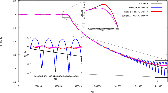
Example output
The picture shows example output, where three different window settings were applied:
While excessive windowing (magenta) reduces stopband ripple, it introduces error at the passband edge that is clearly visible. A small amount of windowing (red) seems like a good compromise, depending on the application.
Causality
”Catch 22” applies (also known as time-bandwidth product): Unless the frequency response |H(f)| of the continuous-time model is essentially zero for frequencies beyond the Nyquist limit, the part of the frequency response cannot be simply discarded. Doing so would implicitly enforce an ideal low-pass filter, which is non-causal and requires an excessive artificial group delay and a very long impulse response to approximate. The situation arises even with a lowpass filter, when modeling at a sampling rate that covers only the passband.
The default solution (unless aliasZones is not set to 0) is to introduce artificial aliasing, which greatly reduces the required impulse response length. Conceptually, it is the same as sampling the continuous-time signal before passing it through the analog component. However, be aware that this may distort the frequency response.
In cases where accuracy is required only within a limited bandwidth - for example, to model filter effects on a received channel that is processed at a fractional oversampling ratio - the option BW_Hz can be used to convert the unused bandwidth into a well-defined raised-cosine filter response.
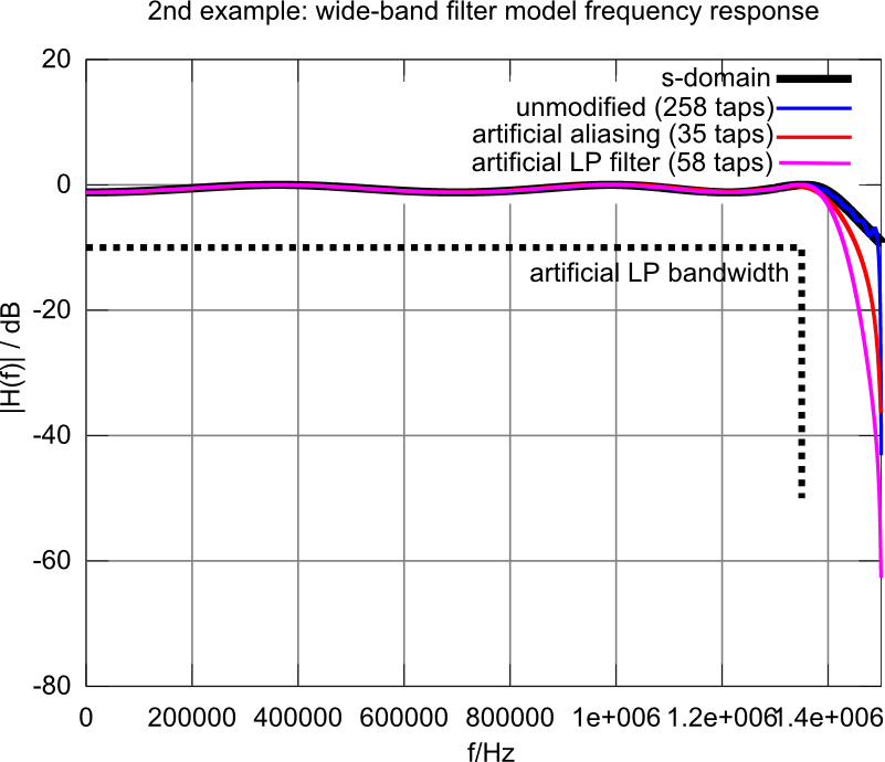
The following pictures shows the frequency response of the resulting model and the required number of FIR taps for
- unmodified truncation of the impulse response (blue)
- artificial aliasing (red, note that the passband is not completely accurate)
- lowpass filtering (magenta).
In any case, the algorithm will insert (or remove) group delay as needed, according to the accuracy target. In other words, relative group delay variations are modeled faithfully, but do not rely on the absolute group delay of the model.
For applications such as control systems where a predictable absolute group delay matters, the algorithm can be trivially modified by assigning a fixed value to ixFirst.
Algorithm
-
Evaluate the frequency response within the given sampling rate, optionally including artificial aliases
-
Apply raised-cosine lowpass filter (optionally)
-
Calculate the impulse response
-
Find the group delay that gives a sufficiently causal impulse response (ixFirst = ...)
-
Truncate the impulse response to a given accuracy target, by default -60 dB relative to the peak sample (ixLast = ...)
-
Apply one-sided raised-cosine windowing
Running the code
Copy into sn_model.m and run sn_model from the command line.
Further development:
If the application requires only part of the bandwidth, it is possible to apply an arbitrary low-pass response on H, for example (root)-raised cosine. This avoids high-frequency "ringing" in the impulse response and may shorten it considerably for a given accuracy threshold. This can be used as alternative to the "artificial aliasing" approach, especially if the model becomes too inaccurate due to the added aliases.
% discrete-time model for Laplace-domain expression
% Markus Nentwig, 30.12.2011
function sn_model()
    close all;
    run_demo1(10);
    run_demo2(11);
end

% ************************************
% Constructs a FIR model for a relatively
% narrow-band continuous-time IIR filter.
% At the edge of the first Nyquist zone
% (+/- fSample/2), the frequency response
% is down by about 70 dB, which makes
% the modeling unproblematic.
% The impact of different windowing options
% is visible both at high frequencies, but
% also as deviation between original frequency
% response and model at the passband edge.
% ************************************
function run_demo1(fig)
    [b, a] = getContTimeExampleFilter();
    fc_Hz = 0.5e6; % frequency corresponding to omegaNorm == 1

    commonParameters = struct(...
        's_a', a, ...
        's_b', b, ...
        'z_rate_Hz', 3e6, ...
        's_fNorm_Hz', fc_Hz, ...
        'fig', fig);

    % sample impulse response without windowing
    ir = sampleLaplaceDomainImpulseResponse(...
        commonParameters, ...
        'plotstyle_s', 'k-', ...
        'plotstyle_z', 'b-');

    % use mild windowing
    ir = sampleLaplaceDomainImpulseResponse(...
        commonParameters, ...
        'plotstyle_z', 'r-', ...
        'winLen_percent', 4);

    % use heavy windowing - error shows at passband edge
    ir = sampleLaplaceDomainImpulseResponse(...
        commonParameters, ...
        'plotstyle_z', 'm-', ...
        'winLen_percent', 100);

    legend('s-domain', 'sampled, no window', 'sampled, 4% RC window', 'sampled, 100% RC window')

    figure(33); clf;
    h = stem(ir);
    set(h, 'markersize', 2);
    set(h, 'lineWidth', 2);
    title('sampled impulse response');
end

% ************************************
% model for a continuous-time IIR filter
% that is relatively wide-band.
% The frequency response requires some
% manipulation at the edge of the Nyquist zone.
% Otherwise, there would be an abrupt change
% that would result in an excessively long impulse
% response.
% ************************************
function run_demo2(fig)
    [b, a] = getContTimeExampleFilter();
    fc_Hz = 1.4e6; % frequency corresponding to omegaNorm == 1

    commonParameters = struct(...
        's_a', a, ...
        's_b', b, ...
        'z_rate_Hz', 3e6, ...
        's_fNorm_Hz', fc_Hz, ...
        'fig', fig);

    % sample impulse response without any manipulations
    ir1 = sampleLaplaceDomainImpulseResponse(...
        commonParameters, ...
        'aliasZones', 0, ...
        'plotstyle_s', 'k-', ...
        'plotstyle_z', 'b-');

    % use artificial aliasing (introduces some passband error)
    ir2 = sampleLaplaceDomainImpulseResponse(...
        commonParameters, ...
        'aliasZones', 5, ...
        'plotstyle_z', 'r-');

    % use artificial low-pass filter (freq. response
    % becomes invalid beyond +/- BW_Hz / 2)
    ir3 = sampleLaplaceDomainImpulseResponse(...
        commonParameters, ...
        'aliasZones', 0, ...
        'BW_Hz', 2.7e6, ...
        'plotstyle_z', 'm-');
    line([0, 2.7e6/2, 2.7e6/2], [-10, -10, -50]);

    legend('s-domain', ...
           sprintf('unmodified (%i taps)', numel(ir1)), ...
           sprintf('artificial aliasing (%i taps)', numel(ir2)), ...
           sprintf('artificial LP filter (%i taps)', numel(ir3)));
    title('2nd example: wide-band filter model frequency response');

    figure(350); grid on; hold on;
    subplot(3, 1, 1);
    stem(ir1, 'b'); xlim([1, numel(ir1)])
    title('wide-band filter model: unmodified');
    subplot(3, 1, 2);
    stem(ir2, 'r');xlim([1, numel(ir1)]);
    title('wide-band filter model: art. aliasing');
    subplot(3, 1, 3);
    stem(ir3, 'm');xlim([1, numel(ir1)]);
    title('wide-band filter model: art. LP filter');
end

% Build example Laplace-domain model
function [b, a] = getContTimeExampleFilter()
    if true
        order = 6;
        ripple_dB = 1.2;
        omegaNorm = 1;
        [b, a] = cheby1(order, ripple_dB, omegaNorm, 's');
    else
        % same as above, if cheby1 is not available
        b =  0.055394;
        a = [1.000000   0.868142   1.876836   1.109439   0.889395   0.279242   0.063601];
    end
end

% ************************************
% * Samples the impulse response of a Laplace-domain
%   component
% * Adjusts group delay and impulse response length so that
%   the discarded part of the impulse response is
%   below a threshold.
% * Applies windowing
%
% Mandatory arguments:
% s_a, s_b:    Laplace-domain coefficients
% s_fNorm_Hz:  normalization frequency for a, b coefficients
% z_rate_Hz:   Sampling rate of impulse response
%
% optional arguments:
% truncErr_dB: Maximum truncation error of impulse response
% nPts:        Computed impulse response length before truncation
% winLen_percent: Part of the IR where windowing is applied
% BW_Hz:       Apply artificical lowpass filter for |f| > +/- BW_Hz / 2
%
% plotting:
% fig:         Figure number
% plotstyle_s: set to plot Laplace-domain frequency response
% plotstyle_z: set to plot z-domain model freq. response
% ************************************
function ir = sampleLaplaceDomainImpulseResponse(varargin)
    def = {'nPts', 2^18, ...
           'truncErr_dB', -60, ...
           'winLen_percent', -1, ...
           'fig', 99, ...
           'plotstyle_s', [], ...
           'plotstyle_z', [], ...
           'aliasZones', 1, ...
           'BW_Hz', []};
    p = vararginToStruct(def, varargin);

    % FFT bin frequencies
    fbase_Hz = FFT_frequencyBasis(p.nPts, p.z_rate_Hz);

    % instead of truncating the frequency response at +/- z_rate_Hz,
    % fold the aliases back into the fundamental Nyquist zone.
    % Otherwise, we'd try to build a near-ideal lowpass filter,
    % which is essentially non-causal and requires a long impulse
    % response with artificially introduced group delay.
    H = 0;
    for alias = -p.aliasZones:p.aliasZones

        % Laplace-domain "s" in normalized frequency
        s = 1i * (fbase_Hz + alias * p.z_rate_Hz) / p.s_fNorm_Hz;

        % evaluate polynomial in s
        H_num = polyval(p.s_b, s);
        H_denom = polyval(p.s_a, s);
        Ha = H_num ./ H_denom;
        H = H + Ha;
    end

    % plot |H(f)| if requested
    if ~isempty(p.plotstyle_s)
        figure(p.fig); hold on; grid on;
        fr = fftshift(20*log10(abs(H) + eps));
        h = plot(fftshift(fbase_Hz), fr, p.plotstyle_s);
        set(h, 'lineWidth', 3);
        xlabel('f/Hz'); ylabel('|H(f)| / dB');
        xlim([0, p.z_rate_Hz/2]);
    end

    % apply artificial lowpass filter
    if ~isempty(p.BW_Hz)
        % calculate RC transition bandwidth
        BW_RC_trans_Hz = p.z_rate_Hz - p.BW_Hz;

        % alpha (RC filter parameter) implements the
        % RC transition bandwidth:
        alpha_RC = BW_RC_trans_Hz / p.z_rate_Hz / 2;

        % With a cutoff frequency of BW_RC, the RC filter
        % reaches |H(f)| = 0 at f = z_rate_Hz / 2
        % BW * (1+alpha) = z_rate_Hz / 2
        BW_RC_Hz = p.z_rate_Hz / ((1+alpha_RC));
        HRC = raisedCosine(fbase_Hz, BW_RC_Hz, alpha_RC);
        H = H .* HRC;
    end

    % frequency response => impulse response
    ir = ifft(H);

    % assume s_a, s_b describe a real-valued impulse response
    ir = real(ir);

    % the impulse response peak is near the first bin.
    % there is some earlier ringing, because evaluating the s-domain
    % expression only for s < +/- z_rate_Hz / 2 implies an ideal,
    % non-causal low-pass filter.

    ir = fftshift(ir);
    % now the peak is near the center

    % threshold for discarding samples
    peak = max(abs(ir));
    thr = peak * 10 ^ (p.truncErr_dB / 20);

    % first sample that is above threshold
    % determines the group delay of the model
    ixFirst = find(abs(ir) > thr, 1, 'first');

    % last sample above threshold
    % determines the length of the impulse response
    ixLast = find(abs(ir) > thr, 1, 'last');

    % truncate
    ir = ir(ixFirst:ixLast);

    % apply windowing
    if p.winLen_percent > 0
        % note: The window drops to zero for the first sample that
        % is NOT included in the impulse response.
        v = linspace(-1, 0, numel(ir)+1);
        v = v(1:end-1);
        v = v * 100 / p.winLen_percent;
        v = v + 1;
        v = max(v, 0);
        win = (cos(v*pi) + 1) / 2;
        ir = ir .* win;
    end

    % plot frequency response, if requested
    if ~isempty(p.plotstyle_z)
        irPlot = zeros(1, p.nPts);
        irPlot(1:numel(ir)) = ir;
        figure(p.fig); hold on;
        fr = fftshift(20*log10(abs(fft(irPlot)) + eps));
        h = plot(fftshift(fbase_Hz), fr, p.plotstyle_z);
        set(h, 'lineWidth', 3);
        xlabel('f/Hz'); ylabel('|H(f)| / dB');
        xlim([0, p.z_rate_Hz/2]);
    end
end

% ************************************
% raised cosine frequency response
% ************************************
function H = raisedCosine(f, BW, alpha)
    c=abs(f * 2 / BW);

    % c=-1 for lower end of transition region
    % c=1 for upper end of transition region
    c=(c-1) / alpha;

    % clip to -1..1 range
    c=min(c, 1);
    c=max(c, -1);

    H = 1/2+cos(pi/2*(c+1))/2;
end

% ************************************
% calculates the frequency that corresponds to each
% FFT bin (negative, zero, positive)
% ************************************
function fb_Hz = FFT_frequencyBasis(n, rate_Hz)
    fb = 0:(n - 1);
    fb = fb + floor(n / 2);
    fb = mod(fb, n);
    fb = fb - floor(n / 2);
    fb = fb / n; % now [0..0.5[, [-0.5..0[
    fb_Hz = fb * rate_Hz;
end

% *************************************************************
% helper function: Parse varargin argument list
% allows calling myFunc(A, A, A, ...)
% where A is
% - key (string), value (arbitrary) => result.key = value
% - a struct => fields of A are copied to result
% - a cell array => recursive handling using above rules
% *************************************************************
function r = vararginToStruct(varargin)
% note: use of varargin implicitly packs the caller's arguments into a cell array
% that is, calling vararginToStruct('hello') results in
%   varargin = {'hello'}
    r = flattenCellArray(varargin, struct());
end

function r = flattenCellArray(arr, r)
    ix=1;
    ixMax = numel(arr);
    while ix <= ixMax
        e = arr{ix};

        if iscell(e)
            % cell array at 'key' position gets recursively flattened
            % becomes struct
            r = flattenCellArray(e, r);
        elseif ischar(e)
            % string => key.
            % The following entry is a value
            ix = ix + 1;
            v = arr{ix};
            % store key-value pair
            r.(e) = v;
        elseif isstruct(e)
            names = fieldnames(e);
            for ix2 = 1:numel(names)
                k = names{ix2};
                r.(k) = e.(k);
            end
        else
            e
            assert(false)
        end
        ix=ix+1;
    end % while
end


