


Introduction to Laplace Transform Analysis
The one-sided Laplace transform of a signal ![]() is defined
by
is defined
by
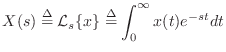
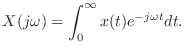
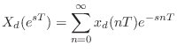
When evaluated along the ![]() axis (i.e.,
axis (i.e., ![]() ), the
Laplace transform reduces to the unilateral Fourier transform:
), the
Laplace transform reduces to the unilateral Fourier transform:
An advantage of the Laplace transform is the ability to transform signals which have no Fourier transform. To see this, we can write the Laplace transform as
![$\displaystyle X(s) = \int_0^\infty x(t) e^{-(\sigma + j\omega)t} dt
= \int_0^\infty \left[x(t)e^{-\sigma t}\right] e^{-j\omega t} dt .
$](http://www.dsprelated.com/josimages_new/filters/img1668.png)
Existence of the Laplace Transform
A functionThe Laplace transform of a causal, growing exponential function
![$\displaystyle x(t) = \left\{\begin{array}{ll}
A e^{\alpha t}, & t\geq 0 \\ [5pt]
0, & t<0 \\
\end{array}\right.,
$](http://www.dsprelated.com/josimages_new/filters/img1674.png)
![\begin{eqnarray*}
X(s) &\isdef & \int_0^\infty x(t) e^{-st}dt
= \int_0^\infty A...
...alpha \\ [5pt]
\infty, & \sigma<\alpha \\
\end{array} \right.
\end{eqnarray*}](http://www.dsprelated.com/josimages_new/filters/img1675.png)
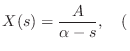
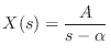
Thus, the Laplace transform of an exponential
![]() is
is
![]() , but this is defined only for
re
, but this is defined only for
re![]() .
.
Analytic Continuation
It turns out that the domain of definition of the Laplace transform can be extended
by means of analytic continuation [14, p. 259].
Analytic continuation is carried out by expanding a function of
![]() about all points in its domain of definition, and
extending the domain of definition to all points for which the series
expansion converges.
about all points in its domain of definition, and
extending the domain of definition to all points for which the series
expansion converges.
In the case of our exponential example
 re
rethe Taylor series expansion of
where, writing ![]() as
as
![]() and using the chain rule for
differentiation,
and using the chain rule for
differentiation,
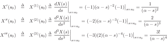
and so on. We also used the factorial notation
![]() , and we defined the special cases
, and we defined the special cases
![]() and
and
![]() , as is normally done.
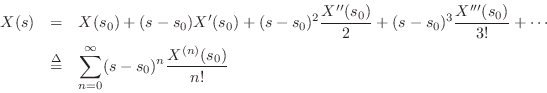
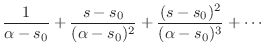
The series expansion of
, as is normally done.
The series expansion of ![]() can thus be written
can thus be written
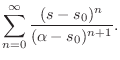
We now ask for what values of ![]() does the series Eq.
does the series Eq.![]() (D.2)
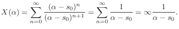
converge? The value
(D.2)
converge? The value ![]() is particularly easy to
check, since
is particularly easy to
check, since
More generally, let's apply the ratio test for the convergence
of a geometric series. Since the ![]() th term of the series is
th term of the series is

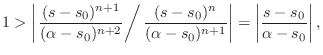
The analytic continuation of the domain of Eq.![]() (D.1) is now
defined as the union of the disks of convergence for all points
(D.1) is now
defined as the union of the disks of convergence for all points
![]() . It is easy to see that a sequence of such disks can
be chosen so as to define all points in the
. It is easy to see that a sequence of such disks can
be chosen so as to define all points in the ![]() plane except at the
pole
plane except at the
pole ![]() .
.
In summary, the Laplace transform of an exponential
![]() is
is
Analytic continuation works for any finite number of poles of finite order,D.2 and for an infinite number of distinct poles of finite order. It breaks down only in pathological situations such as when the Laplace transform is singular everywhere on some closed contour in the complex plane. Such pathologies do not arise in practice, so we need not be concerned about them.
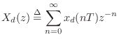
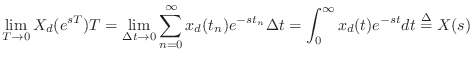
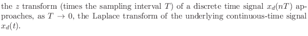
Relation to the z Transform
The Laplace transform is used to analyze continuous-time
systems. Its discrete-time counterpart is the ![]() transform:
transform:
In summary,
Note that the ![]() plane and
plane and ![]() plane are generally related by
plane are generally related by
Laplace Transform Theorems
Linearity
The Laplace transform is a linear operator. To show this, let
![]() denote a linear combination of signals
denote a linear combination of signals ![]() and
and ![]() ,
,
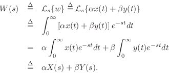
Thus, linearity of the Laplace transform follows immediately from the linearity of integration.
Differentiation
The differentiation theorem for Laplace transforms states that
Proof:
This follows immediately from integration by parts:
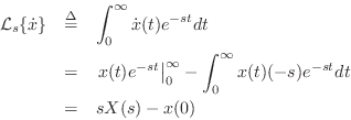
since
![]() by assumption.
by assumption.
Corollary: Integration Theorem
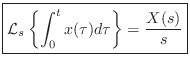
Thus, successive time derivatives correspond to successively higher
powers of ![]() , and successive integrals with respect to time
correspond to successively higher powers of
, and successive integrals with respect to time
correspond to successively higher powers of ![]() .
.
Laplace Analysis of Linear Systems
The differentiation theorem can be used to convert differential equations into algebraic equations, which are easier to solve. We will now show this by means of two examples.
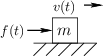
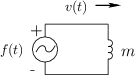
Moving Mass
Figure D.1 depicts a free mass driven by an external force along
an ideal frictionless surface in one dimension. Figure D.2
shows the electrical equivalent circuit for this scenario in
which the external force is represented by a voltage source emitting
![]() volts, and the mass is modeled by an inductor
having the value
volts, and the mass is modeled by an inductor
having the value ![]() Henrys.
Henrys.
From Newton's second law of motion ``![]() '', we have
'', we have
![\begin{eqnarray*}
F(s) &=& m\,{\cal L}_s\{{\ddot x}\}\\
&=& m\left[\,s {\cal L...
...right\}\\
&=& m\left[s^2\,X(s) - s\,x(0) - {\dot x}(0)\right].
\end{eqnarray*}](http://www.dsprelated.com/josimages_new/filters/img1738.png)
Thus, given
 Laplace transform of the driving force
  ,
,
 initial mass position, and
-
 initial mass velocity,
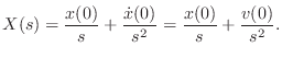
If the applied external force ![]() is zero, then, by linearity of
the Laplace transform, so is
is zero, then, by linearity of
the Laplace transform, so is ![]() , and we readily obtain
, and we readily obtain
![$\displaystyle u(t)\isdef \left\{\begin{array}{ll}
0, & t<0 \\ [5pt]
1, & t\ge 0 \\
\end{array}\right.,
$](http://www.dsprelated.com/josimages_new/filters/img1745.png)
To summarize, this simple example illustrated use the Laplace transform to solve for the motion of a simple physical system (an ideal mass) in response to initial conditions (no external driving forces). The system was described by a differential equation which was converted to an algebraic equation by the Laplace transform.
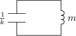
Mass-Spring Oscillator Analysis
Consider now the mass-spring oscillator depicted physically in Fig.D.3, and in equivalent-circuit form in Fig.D.4.
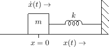 |
By Newton's second law of motion, the force ![]() applied to a mass
equals its mass times its acceleration:
applied to a mass
equals its mass times its acceleration:
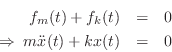
We have thus derived a second-order differential equation governing
the motion of the mass and spring. (Note that ![]() in
Fig.D.3 is both the position of the mass and compression
of the spring at time
in
Fig.D.3 is both the position of the mass and compression
of the spring at time ![]() .)
.)
Taking the Laplace transform of both sides of this differential equation gives
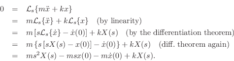
To simplify notation, denote the initial position and velocity by
![]() and
and
![]() , respectively. Solving for
, respectively. Solving for ![]() gives
gives
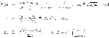
denoting the modulus and angle of the pole residue ![]() , respectively.
From §D.1, the inverse Laplace transform of
, respectively.
From §D.1, the inverse Laplace transform of ![]() is
is
![]() , where
, where ![]() is the Heaviside unit step function at time 0.
Then by linearity, the solution for
the motion of the mass is
is the Heaviside unit step function at time 0.
Then by linearity, the solution for
the motion of the mass is
![\begin{eqnarray*}
x(t) &=& re^{-j{\omega_0}t} + \overline{r}e^{j{\omega_0}t}
= ...
...ga_0}t - \tan^{-1}\left(\frac{v_0}{{\omega_0}x_0}\right)\right].
\end{eqnarray*}](http://www.dsprelated.com/josimages_new/filters/img1771.png)
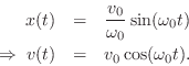
If the initial velocity is zero (![]() ), the above formula
reduces to
), the above formula
reduces to
![]() and the mass simply oscillates sinusoidally at frequency
and the mass simply oscillates sinusoidally at frequency
![]() , starting from its initial position
, starting from its initial position ![]() .
If instead the initial position is
.
If instead the initial position is ![]() , we obtain
, we obtain
Next Section:
Analog Filters
Previous Section:
Allpass Filters


