


Frequency-Dependent Damping
In real vibrating strings, damping typically increases with frequency
for a variety of physical reasons
[73,77]. A simple
modification [392] to Eq.![]() (6.14) yielding
frequency-dependent damping is
(6.14) yielding
frequency-dependent damping is
The result of adding such damping terms to the wave equation is that
traveling waves on the string decay at frequency-dependent
rates. This means the loss factors ![]() of the previous section
should really be digital filters having gains which decrease
with frequency (and never exceed
of the previous section
should really be digital filters having gains which decrease
with frequency (and never exceed ![]() for stability of the loop).
These filters commute with delay elements because they are
linear and time invariant (LTI) [449]. Thus,
following the reasoning of the previous section, they can be lumped at
a single point in the digital waveguide. Let
for stability of the loop).
These filters commute with delay elements because they are
linear and time invariant (LTI) [449]. Thus,
following the reasoning of the previous section, they can be lumped at
a single point in the digital waveguide. Let
![]() denote the
resulting string loop filter (replacing
denote the
resulting string loop filter (replacing ![]() in
Fig.6.127.7). We have the stability (passivity)
constraint
in
Fig.6.127.7). We have the stability (passivity)
constraint
![]() , and making the filter
linear phase (constant delay at all frequencies) will restrict
consideration to symmetric FIR filters only.
, and making the filter
linear phase (constant delay at all frequencies) will restrict
consideration to symmetric FIR filters only.
Restriction to FIR filters yields the important advantage of keeping the approximation problem convex in the weighted least-squares norm. Convexity of a norm means that gradient-based search techniques can be used to find a global miminizer of the error norm without exhaustive search [64],[428, Appendix A].
The linear-phase requirement halves the degrees of freedom in the filter
coefficients. That is, given
![]() for
for ![]() , the coefficients
, the coefficients
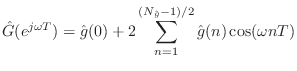
![]() are also determined. The loss-filter frequency response
can be written in terms of its (impulse response) coefficients as
are also determined. The loss-filter frequency response
can be written in terms of its (impulse response) coefficients as
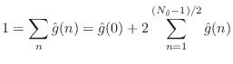
A further degree of freedom is eliminated from the loss-filter
approximation by assuming all losses are insignificant at 0 Hz so that
![]() (taking the approximation error to be zero at
(taking the approximation error to be zero at
![]() ). This means the coefficients of the FIR filter must sum to
). This means the coefficients of the FIR filter must sum to ![]() .
If the length of the filter is
.
If the length of the filter is
![]() , we have
, we have
Next Section:
The Stiff String
Previous Section:
The Damped Plucked String


