Hi,  

I am inputting a 100hz sine wave into a low pass filter.  I am sampling at 44800hz.  One thing I am noticing is that when decimation by lets say 2.  I set the lowpass filter cutoff to 44800/4.  

however when doing this.. the FFT frequency of the input wave shows 50hz instead of 100.  

Any ideas?

Thanks!

Mike

When you decimate, you increase the sample interval.  The sample interval is used in determining the spectrum.  When you increase the sample interval by a factor of 2, you have to change the code to give the correct frequency value.

I think you've inadvertently quartered the original sample rate instead of using half the original sample rate of 44.8 kHz.

Consider this example,

close all; clear; clc;
set( 0, 'DefaultFigureWindowStyle', 'docked' );

fs = 44.8e3;

netTime = 1;
    timeIndices = 0:1/fs:(netTime - 1/fs);
    
f = 100;
    s = sin( 2 .* pi .* f .* timeIndices );
    
[ MX, f ] = fourier( s, fs, 16384 );  % Bin resolution:  2.73 Hz
%     figure; plot( f, 20*log10(MX) ); grid on; xlim( [ min(f) max(f) ] ); shg;
    
y = resample(s, 1, 2);
    [ MX, f ] = fourier( y, fs/2, 16384 );  % Bin resolution:  1.37 Hz
%         figure; plot( f, 20*log10(MX) ); grid on; xlim( [ min(f) max(f) ] ); shg;
        
[ b, a ] = butter( 6, (fs/4)/(fs/2), 'low' );
    figure; freqz( b, a, 4096, fs/4 );
    figure; zplane( b, a );
    
yf = filter( b, a, y );
    [ MX1, f1 ] = fourier( yf, fs/4, 16384 );  % Bin resolution:  0.68 Hz
    [ MX2, f2 ] = fourier( yf, fs/2, 16384 );  % Bin resolution:  1.37 Hz
        figure; ...
            plot( f1, 20*log10(MX1) ); grid on; xlim( [ min(f1) max(f1) ] ); hold on;
            plot( f2, 20*log10(MX2) ); grid on; xlim( [ min(f2) max(f2) ] ); shg;
            xlabel('Frequency (Hz)'); ylabel('Magnitude (dB)'); axis( [0 2e3 -20 0] );
            legend('fs/4', 'fs/2');  shg;

digital frequency is 2*pi*(fc/fs) with units of radians per sample if you reduce the sample rate by 2 the digital freq is 2*pi*(fc/(fs/2)) with units of radians/sample so the digital freq has changed has doubled ... if it was rotating 10 degrees per sample at the input rate it is nor rorating at 20 degrees per sample because the sample interval has doubled..

if we multiply the digital frequency by the sample rate we convert from dig freq to analog freq since the digital freq doubled and the sample rate halved, the product is the same in the two sample rates.

best regards

fred h

Hi,

The sketch shows how the spectra of the signals change through the filtering and downsample.

In the illustration a) the original spectrum is shown. It contains the useful signal of the frequency fsig and a disturbance

In b) the amplitude response of the low-pass filter is shown as a decimation filter.

The spectrum after filtering is shown in c). The disturbance is removed.

In d) the spectrum after the downsample with a factor 2 is shown.

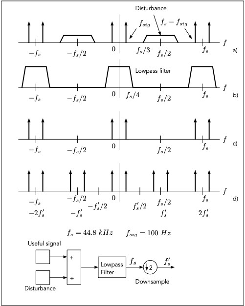
As you can see the signal still has the same frequency of 100 Hz but with a lower sampling frequency of fs' = 44.8 / 2 kHz.

The facts can be easily explained with a small Simulink model (Fig. 1).

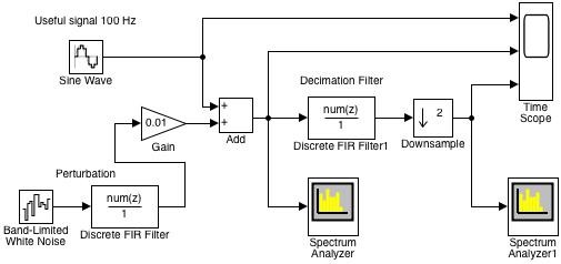
Fig. 1 Simulink model of the decimation

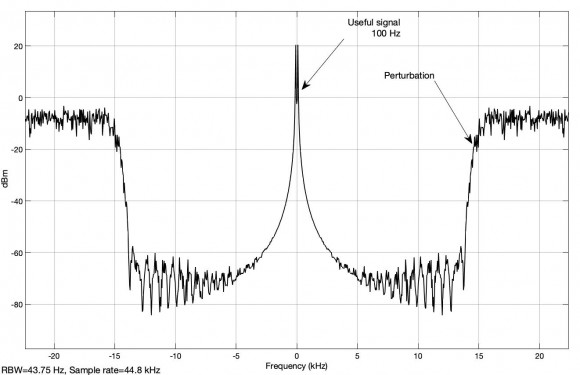
The useful signal and the disturbance are added at the input. They are sampled at 44.8 kHz. The spectrum of these signals is shown in Fig. 2 shown. 

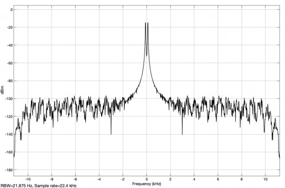
After filtering, the interference is suppressed and the spectrum from Fig. 3 is obtained after the downsample. It now represents the useful signal without interference.

The signals are shown on the scope block (Fig. 3):

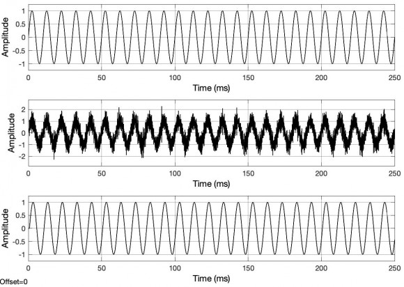
Right at the top the useful signal without interference

In the middle the useful signal with interference

At the bottom the signal after the decimation.

Regards

Probably replicating all the fine answers already, but when considering these types of situations, I always remember my golden rule of spectrum analysis:

    bin size = ( ( 2 * PI ) / ( # of FFT points ) )

where ( 2 * PI ) is the signal rate, i.e. initially 44800 Hz in your case, decimated to 22400 Hz.  Assuming ( # of FFT points ) didn't change, decimation by 2 cuts that ratio in half.  So the same bin location will be half the frequency of before.  But there shouldn't really be any signal component there, at the original bin location ... call it bin X, after decimation.  It should have moved closest to twice that original bin X from before decimation.  

A simple example for illustration and explaining "closest":

    initial sample rate 44800 Hz

    signal @ 100 Hz

    fft size = 512

bin size will be ( 44800 / 512 ) = 87.5

0th bin is DC, 1st bin is 87.5 Hz, 2nd bin is 175 Hz.  So the 100 Hz signal will appear between the 1st and 2nd bin, biased towards first one (since closer to 100 Hz)

Now, with decimation by 2

    sample rate = 22400 Hz

    signal @ 100 Hz

    fft size = 512

bin size will be ( 22400 / 512 ) = 43.75

first bin is DC, 1st bin is 43.75, 2nd bin is 87.5, 3rd bin is 131.25.  So the 100 Hz signal will appear between the 2nd and 3rd bin, closest to the 2nd bin, but more component of it, in the neighboring bin (3rd) this time, since that neighbor bin is not as far away from 100 Hz as the neighbor bin was before decimation.

Unless you signal is an exact multiple of the bin size, you will get "smear" across the bins closest to the signal frequency.

Regards,

Robert

I'm just curious how someone ends up with a 44800 Hz sample rate.  :)