Hi all

I am simulating signals on two hydrophones H1 and H2 of linear array which are at a distance 'd' from each other. The geometry is shown below:

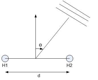
Assuming Plane Wave assumption, there will be some delay b/w signals arriving at H1 and H2 assuming zero noise and pure sinusoidal signals. After simulating the signals with delays, I am trying to calculate back the delay using MATLAB 'gccphat' function, but its output does not match with the delay simulated in signals? MATLAB code is given below:

---

---

clc

clear

close all

%%%%=======================================================================

%%%%============================General Parameters=========================

%%%%=======================================================================

total_sens=2;

fo=8500;%frequency in Hz

samp_f=30*51.2e3;%Sampling frequency

samp_t=1/samp_f;

chunk_size=163840;

total_chunks=1;

chunk_time=chunk_size/samp_f;

chunk_t=0:samp_t:(samp_t*(chunk_size-1));%time vector calculated

c=1500;%speed of sound

%%%%=======================================================================

%%%%=====================DA PRA Array Parameters===========================

%%%%=======================================================================

D=15;%separation b/w sensors in m

Target_theta=40;%Source angle in deg

delay_=D*sind(Target_theta)/c

H1(1:chunk_size,1)=sin(2*pi*fo*(chunk_t))+0*randn(1,chunk_size);%Sensor H1 signal

H2(1:chunk_size,1)=sin(2*pi*fo*(chunk_t+delay_))+0*randn(1,chunk_size);%Sensor H2 signal

% figure,plot(H1(1:2000)),hold on,plot(H2(1:2000),'r')

tau12=gccphat(H1,H2,samp_f)

---

---

The simulated delay_ is approx. 0.0064s whereas delay calculated by 'gccphat is 0s??.

Kindly help me in this regard. Thanks

Hi, your approach is right and cross correlation can be used to estimate delay between 2 signals. but to get the right peak you need to take envelope.

n0 = 1;
n1= floor(samp_f/fo);
n2= 4*n1-1;
  
S1 = H1(n0:n2);
S2 = H2(n0:n2);
  
%tau12=gcc_phat(S1, S2,samp_f)
tau13=delay_estimate(S1, S2, samp_f)
tau4 = finddelay(S1, S2) / samp_f

function td = delay_estimate(x1, x2, fs)
  r = abs(hilbert(xcorr(x1,x2)));
  [a,i] = max(r);
  td = i - length(r)/2; 
  plot(r);
endfunction

finddelay() based estimate is giving close values with reduced sample count to estimator. 

taking envelope of the xcorr is also expected give more accurate result for non-cyclic signals such as chirp.  delay_estimate() added above. 

Hope it helps. 

Regards,

Chalil

Hi Chalil

Thanks very much for help. I have used your kind advise but still the delays measured by your 'delay_estimate' function or MATLAB 'finddelay' function i.e. -3.255e-07s & -1.6276e-05s are far away than the actual delay i introduced (simulate) in the signals i.e. 0.0064s?

Regards

Hi, Looks like the the frequency of tone you're using is higher. if i use a lower freq the results are ok. yet to fully understand the theory.

updated code : 

...

fo=40 
...

tau13=delay_estimate(S1, S2, samp_f)
tau4 = finddelay(S1, S2) / samp_f

function td = delay_estimate(x1, x2, fs)
%  r = abs(hilbert(xcorr(x1,x2)));
  r = abs(xcorr(x1,x2));
  [a,i] = max(r);
  td = (i - length(r)/2)/fs; 
  plot(r);
endfunction

for d = 10

delay_ = 4.2853e-03

tau13 = 4.2370e-03

tau4 = -4.2344e-03

Hi Chalil

Thanks for help. I am lost here somehow that why correlation results are depending upon frequency of signals? Let us forget about 2 sensors geometry, i simply generate two sinusoidal signals of same frequency, i introduce a fixed delay in one of the signals and then correlate them. As per my understanding, correlation peak should correspond to the delay introduced whether it is being calculated through 'gccphat' or 'finddelay' or 'delay_estimate' functions.

 Can there be a problem in a way i am generating two sinusoidal signals and introducing the delay?

Thanks

Hello naumankalia, i checked the code where you're generating two sinusoidal signals and introducing the delay. it looks fine. 

one point is that if you want to check delay larger than 'D' the period of the signal shall be larger than that. 

function [delay_act, delay_est] = tst2(d)
  fs = 192e3;     % Hz
  fo = 50;         % freq 
  duration = 2^18/fs;   % time  in Sec
  
  samples = fs*duration;
  t_idx = 0:samples-1;
  t = t_idx;
  
  x = cos(2*pi*fo*t/fs);
  y = cos(2*pi*fo*(t-d)/fs); % +0.25*randn(size(samples));
   
  delay_act = d/fs;
  len = (fs/fo)*2;    % no  need to pass full signal to xcorr. pass only 1-4 cycles 
   
  [xc,lags] = xcorr(y,x,len,'coeff');


  subplot(2,1,1);
  plot(y, 'r'); hold;
  plot(x, 'g'); hold;
  
  subplot(2,1,2);
  plot(lags,xc); hold;


  [max_v, max_i] = max(xc);
  
  delay_est_idx = max_i-len;
  plot(delay_est_idx, max_v, 'x'); hold;
  printf(' delay = %f Sec actual delay = %f\n', delay_est_idx/fs, delay_act);
  printf(' delay = %d Sec actual delay = %d\n', delay_est_idx, d);
  
  delay_est = delay_est_idx/fs;
endfunction

the above tst code can be used to check delay estimated against actual. the fs, fo can be configured in the code. 

>> [a, b] = tst2(40)
delay = 0.000208 Sec actual delay = 0.000208
delay = 40 Samples actual delay = 40 Samples 

now for a higher delay the results is : 

>> [a, b] = tst2(4000)
 delay = 0.000833 Sec actual delay = 0.020833
 delay = 160 Samples actual delay = 4000 Samples

the results of not correct. now, reduce the fo = 20 the new results is : 

[a, b] = tst2(4000)
 delay = 0.020766 Sec actual delay = 0.020833
 delay = 3987 Samples actual delay = 4000 Samples

Note : if you use chirp  instead of sine, the results are going to be better as the peak in the xcorr output will hold more energy and side lobs are going to be much shorter than that with sine tone. 

to check you can replace H1 and H2 with :

H1 = chirp (chunk_t, fo, chunk_time, chirp_n*fo);
H2 = chirp (chunk_t+delay_, fo, chunk_time, chirp_n*fo);

hope it helps.

- Chalil

Hello naumankalia,

Unfortunately I am using an older version of Matlab and cannot use the gccphat function, but if you calculate the cross correlation of two sinusoidal signals you get many maxima and minima with equal values. This may be the problem. 

I would like to make a further comment: In your code you have set a distance of 15 m between the two pressure sensors. At the same time you simulate a time harmonic excitation of the medium (presumably water) with a frequency of 8500 Hz assuming a sound velocity of 1500m/s. Thus, with your simulation setup you are violating the spatial sampling theorem. Your sensors should be less than wavelength/2 apart for localization calculations. In your example, this is less than 8.8cm.

Many greetings

Hello mospel

Thanks for reply. yes your are right but wavelength/2 spacing is requirement of standard beam forming techniques. Here the problem i am facing is somewhat different. 

Let us forget about 2 sensors geometry, i simply generate two sinusoidal signals of same frequency, i introduce a fixed delay in one of the signals and then correlate them. As per my understanding, correlation peak should correspond to the delay introduced whether it is being calculated through MATLAB 'gccphat' or 'finddelay' functions.

Thanks

Hello,

If these signals are pure sinusoidal and they are the same frequency then you can estimate the time difference by a difference in phase.

One way would be to take a Hilbert transform of each waveform to get the quadrature signal.  Then ATAN2 of each waveform to get the phase.

The delta phase in the frequency domain can be related back to delta time in the time domain.

Averaging Delta Phase over many point pairs would help with noise if there is any.

As someone else mentioned another problem for ranging is to be sure you are looking in the right cycle of the sinusoid.  The cross-correlation of the magnitude of the output of the Hilbert transform can help you get on the right cycle. (Maybe look at some point in the power rise-time?) Then the phase can give you the fine measurement.

Have fun,

Mark Napier

Hi,

Thanks for help. Yes, you are right. There are multiple ways to find delay b/w two signals but currently i am interested in measuring delay using correlation method. I have also tried Hilbert transform method as suggested, but can not get the desired results.

Thanks

Unfortunately for this situation, I'm not a MATLAB user, nor can I tell how dedicated you are to applying the "gccphat" function.

Presuming you want the answer to "What is the best way to calculate the phase difference in this situation?"

You said simulating, so quality and noise presence is under your determination.  Thus you should expect an exact solution is possible, meaning one that isn't an approximation.

It seems you know the frequency ahead of time, which makes things easier.  The following should be readily implementable in MATLAB, and if you do so, please post the results.

Select a sample frame length which contains a whole number of cycles (w) plus a half.  This technique's accuracy depends on the signal waves being fairly uniform over the frame.  The number of samples should be approximately four per cycle.  The more noise, and the smaller your whole cycle count is, the denser you will want to sample.

Calculate the four DFT bin values around your whole and a half value.  These are complex values, so build a complex vector.

Z[1] = DFT[k=w-1]
Z[2] = DFT[k=w]
Z[3] = DFT[k=w+1]
Z[4] = DFT[k=w+2]

Now, if you have about 4 samples per cycle, your bins are at the half Nyquist point of the spectrum, and the distinction between complex tones and real tones is as minimal as it gets.  Therefore, you are like to get just as good for the job values using the complex tone model, not the real tone model.

Next, for complex tones, build a basis vector using your known frequency and the formula for bin values for pure tones.

Y[1] = BinValue[f,phi=0,k=w-1]
Y[2] = BinValue[f,phi=0,k=w]
Y[3] = BinValue[f,phi=0,k=w+1]
Y[4] = BinValue[f,phi=0,k=w+2]

The rest is straightforward linear algebra.

Z = q Y

ZY* = q YY*

q = (ZY*) / (YY*)

YY* will be real.

q = M e^(i phi)

M = |q|

phi = atan2(q_imag,q_eal)

See: Phase and Amplitude Calculation for a Pure Complex Tone in a DFT using Multiple Bins

For real tones, the process is similar, but two basis vectors need to be used.

See: Phase and Amplitude Calculation for a Pure Real Tone in a DFT: Method 1

From there, you will still need to convert the phase difference to a distance difference.

See: DFT exercise in the book Understanding digital signal processing 3 Ed

Including accounting for "wrapping".  This method will be good at filtering out other tones that may be present and should be very noise robust as well.

If you source is moving, you may wish to do a frequency calculation as well.  With a high quality signal, the Doppler effect calculations should be pretty accurate.

At 8500 Hz tone:

1/8500 = 0.000117647 seconds per cycle

0.0064 seconds per delay (your figure)

0.0064 / (1/8500) = 54.4 cycles per delay (wrappings)

Perhaps you should include a low reference tone for ranging, then use the high tone for precision.  I'll bet even in free air, you can measure something to within a very precise location this way, or at least change in position.

Hi Cedron

Can you kindly explain further the calculations you have done above? How these effect correlation results?

Thanks

When you have a pure tone in a signal frame, the DFT spectrum follows a pattern.  For any tone, the results are proportional to the input tone in terms of any real scalar coefficient.  For complex pure tones, that is also true for complex numbers.  Any real tone defined as x[n] = A e^i(omega*n+phi) can be defined as x[n] = [Ae^i(phi)] * e^i(omega*n)

As a result, if you artificially construct the DFT for the signal tone definition part on the right side, and use the calculated DFT on the signal on the left.  The value of [Ae^i(phi)] can be calculated from each and every bin.  However, only the bins near the peak bin are going to have high SNR values compared to the rest.

Treating a subset of bins as a vector allows you to find the "best fit" ratio as a weighted average of the ratios for bins you selected.  Since the DFT is very good at filtering out other tones and noise in general, this will give you good results.

A real valued signal isn't as simple.  But the rotation rule is still true in the vicinity, approximately.  However, since there are actually two tones at play (one at the frequency, one at the negative frequency), having exact formulas to calculate the DFT (without doing the summation) allows you to do the same trick with two basis vectors to get the same accuracy in results.

If you have no other signals, and have that many wrappings in your delay, I would go with kaz's suggestion of sending a frequency varying chirp so you can align it properly in the time domain.

Hi Cedron

Thanks very much for help. Presently, i am only interested using correlation method.

Thanks

Without going into details that I don't have experience in, my only comment is that the "plane wave" assumption is based on a far field signal and not a near field signal. Like RF (where I have a little experience), the distinction and be significant. Also in
RF, propagation delay is small since things move near the speed of light, simplifies a lot of calculations. So, for example, the distance to the source of the plane wave has to be orders of magnitude greater than the distance between hydrophones. So, while the speed of sound in water is nearly 5 times that in air, it's still pretty slow compared to light. And, this is a 4 dimensional problem, not 3 (but that may be my inexperience speaking).

Using single tones is not best way to test delay as the peak of correlation is very gradual.

Use following frequency sweep (y). The correlation peak is unmistakable.

L = 839;

y = exp(-j*pi/L*(0:L-1).*(1:L));

y_d = [0 y(1:end-1)]; %example delay/advance

%check peak:

test1 = xcorr(y,y);

test2 = xcorr(y,y_d);