


Constant Resonance Gain
It turns out it is possible to normalize exactly the
resonance gain of the second-order resonator tuned by a
single coefficient [89]. This is accomplished by
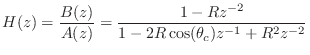
placing the two zeros at
![]() , where
, where ![]() is the radius of
the complex-conjugate pole pair . The transfer function numerator
becomes
is the radius of
the complex-conjugate pole pair . The transfer function numerator
becomes
![]() , yielding
the total transfer function
, yielding
the total transfer function
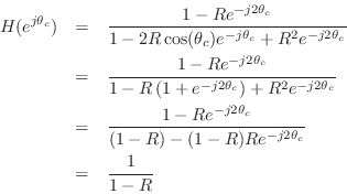
Thus, the gain at resonance is ![]() for all resonance tunings
for all resonance tunings ![]() .
.
Figure B.19 shows a family of amplitude responses for the
constant resonance-gain two-pole, for various values of ![]() and
and
![]() . We see an excellent improvement in the regularity of the
amplitude response as a function of tuning.
. We see an excellent improvement in the regularity of the
amplitude response as a function of tuning.
![\includegraphics[width=\twidth ]{eps/cgresgain}](http://www.dsprelated.com/josimages_new/filters/img1523.png) |
Next Section:
Peak Gain Versus Resonance Gain
Previous Section:
Normalizing Two-Pole Filter Gain at Resonance


