


Normalizing Two-Pole Filter Gain at Resonance
The question we now pose is how to best compensate the tunable
two-pole resonator of §B.1.3 so that its peak gain is the same for
all tunings. Looking at Fig.B.17, and remembering the graphical
method for determining the amplitude response,B.6 it is intuitively
clear that we can help matters by adding two zeros to the
filter, one near dc and the other near ![]() . A zero exactly at dc
is provided by the term
. A zero exactly at dc
is provided by the term
![]() in the transfer function numerator.
Similarly, a zero at half the sampling rate is provided by the term
in the transfer function numerator.
Similarly, a zero at half the sampling rate is provided by the term
![]() in the numerator. The series combination of both zeros
gives the numerator
in the numerator. The series combination of both zeros
gives the numerator
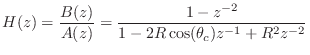
![]() . The complete
second-order transfer function then becomes
. The complete
second-order transfer function then becomes
Checking the gain for the case
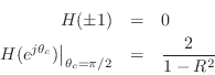
which is better behaved, but now the response falls to zero at dc and
![]() rather than being heavily boosted, as we found in
Eq.
rather than being heavily boosted, as we found in
Eq.![]() (B.12).
(B.12).
Next Section:
Constant Resonance Gain
Previous Section:
DC Blocker Software Implementations


