


Difference Equation
The difference equation is a formula for computing an output
sample at time ![]() based on past and present input samples and past
output samples in the time domain.6.1We may write the general, causal, LTI difference equation as follows:
based on past and present input samples and past
output samples in the time domain.6.1We may write the general, causal, LTI difference equation as follows:
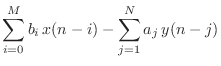
where
As a specific example, the difference equation
When the coefficients are real numbers, as in the above example, the filter is said to be real. Otherwise, it may be complex.
Notice that a filter of the form of Eq.![]() (5.1) can use ``past''
output samples (such as
(5.1) can use ``past''
output samples (such as ![]() ) in the calculation of the
``present'' output
) in the calculation of the
``present'' output ![]() . This use of past output samples is called
feedback. Any filter having one or more
feedback paths (
. This use of past output samples is called
feedback. Any filter having one or more
feedback paths (![]() ) is called
recursive. (By
the way, the minus signs for the feedback in Eq.
) is called
recursive. (By
the way, the minus signs for the feedback in Eq.![]() (5.1) will be
explained when we get to transfer functions in §6.1.)
(5.1) will be
explained when we get to transfer functions in §6.1.)
More specifically, the ![]() coefficients are called the
feedforward coefficients and the
coefficients are called the
feedforward coefficients and the ![]() coefficients are called
the feedback coefficients.
coefficients are called
the feedback coefficients.
A filter is said to be recursive if and only if ![]() for
some
for
some ![]() . Recursive filters are also called
infinite-impulse-response (IIR) filters.
When there is no feedback (
. Recursive filters are also called
infinite-impulse-response (IIR) filters.
When there is no feedback (
![]() ), the filter is said
to be a nonrecursive or
finite-impulse-response (FIR) digital filter.
), the filter is said
to be a nonrecursive or
finite-impulse-response (FIR) digital filter.
When used for discrete-time physical modeling, the difference equation may be referred to as an explicit finite difference scheme.6.2
Showing that a recursive filter is LTI (Chapter 4) is easy by considering its impulse-response representation (discussed in §5.6). For example, the recursive filter
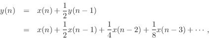
has impulse response
![]() ,
,
![]() . It is now
straightforward to apply the analysis of the previous chapter to find
that time-invariance, superposition, and the scaling property hold.
. It is now
straightforward to apply the analysis of the previous chapter to find
that time-invariance, superposition, and the scaling property hold.
Next Section:
Signal Flow Graph
Previous Section:
Linearity and Time-Invariance Problems


