


Linear Time-Invariant Digital Filters
In this chapter, the important concepts of linearity and time-invariance (LTI) are discussed. Only LTI filters can be subjected to frequency-domain analysis as illustrated in the preceding chapters. After studying this chapter, you should be able to classify any filter as linear or nonlinear, and time-invariant or time-varying.
The great majority of audio filters are LTI, for several reasons: First, no new spectral components are introduced by LTI filters. Time-varying filters, on the other hand, can generate audible sideband images of the frequencies present in the input signal (when the filter changes at audio rates). Time-invariance is not overly restrictive, however, because the static analysis holds very well for filters that change slowly with time. (One rule of thumb is that the coefficients of a quasi-time-invariant filter should be substantially constant over its impulse-response duration.) Nonlinear filters generally create new sinusoidal components at all sums and differences of the frequencies present in the input signal.5.1This includes both harmonic distortion (when the input signal is periodic) and intermodulation distortion (when at least two inharmonically related tones are present). A truly linear filter does not cause harmonic or intermodulation distortion.
All the examples of filters mentioned in Chapter 1 were LTI, or
approximately LTI. In addition, the ![]() transform and all forms of the
Fourier transform are linear operators, and these operators can be
viewed as LTI filter banks, or as a single LTI filter having
multiple outputs.
transform and all forms of the
Fourier transform are linear operators, and these operators can be
viewed as LTI filter banks, or as a single LTI filter having
multiple outputs.
In the following sections, linearity and time-invariance will be formally introduced, together with some elementary mathematical aspects of signals.
Definition of a Signal
Mathematically, we typically denote a signal as a real- or complex-valued function of an integer, e.g.,
Definition. A real discrete-time signal is defined as any time-ordered sequence of real numbers. Similarly, a complex discrete-time signal is any time-ordered sequence of complex numbers.
Using the set notation
![]() , and
, and ![]() to denote
the set of all integers, real numbers, and complex numbers,
respectively, we can express that
to denote
the set of all integers, real numbers, and complex numbers,
respectively, we can express that ![]() is a real, discrete-time signal
by expressing it as a function mapping every integer (optionally in
a restricted range) to a real number:
is a real, discrete-time signal
by expressing it as a function mapping every integer (optionally in
a restricted range) to a real number:
Similarly, a discrete-time complex signal is a mapping from each integer to a complex number:
It is useful to define ![]() as the signal space consisting
of all complex signals
as the signal space consisting
of all complex signals
![]() ,
,
![]() .
.
We may expand these definitions slightly to include functions of the
form ![]() ,
, ![]() , where
, where
![]() denotes the sampling
interval in seconds. In this case, the time index has physical units
of seconds, but it is isomorphic to the integers. For finite-duration
signals, we may prepend and append zeros to extend its domain to all
integers
denotes the sampling
interval in seconds. In this case, the time index has physical units
of seconds, but it is isomorphic to the integers. For finite-duration
signals, we may prepend and append zeros to extend its domain to all
integers ![]() .
.
Mathematically, the set of all signals ![]() can be regarded a
vector space5.2
can be regarded a
vector space5.2 ![]() in
which every signal
in
which every signal ![]() is a vector in the space (
is a vector in the space (
![]() ). The
). The
![]() th sample of
th sample of ![]() ,
, ![]() , is regarded as the
, is regarded as the ![]() th vector
coordinate. Since signals as we have defined them are infinitely
long (being defined over all integers), the corresponding vector space
th vector
coordinate. Since signals as we have defined them are infinitely
long (being defined over all integers), the corresponding vector space
![]() is infinite-dimensional. Every vector space comes with
a field of scalars which we may think of as constant gain
factors that can be applied to any signal in the space. For purposes
of this book, ``signal'' and ``vector'' mean the same thing, as do
``constant gain factor'' and ``scalar''. The signals and gain factors
(vectors and scalars) may be either real or complex, as applications
may require.
is infinite-dimensional. Every vector space comes with
a field of scalars which we may think of as constant gain
factors that can be applied to any signal in the space. For purposes
of this book, ``signal'' and ``vector'' mean the same thing, as do
``constant gain factor'' and ``scalar''. The signals and gain factors
(vectors and scalars) may be either real or complex, as applications
may require.
By definition, a vector space is closed under linear
combinations. That is, given any two vectors
![]() and
and
![]() , and any two scalars
, and any two scalars ![]() and
and ![]() , there exists a
vector
, there exists a
vector
![]() which satisfies
which satisfies
![]() , i.e.,
, i.e.,
A linear combination is what we might call a mix of two signals
![]() and
and ![]() using mixing gains
using mixing gains ![]() and
and ![]() (
(
![]() ). Thus, a signal mix is represented
mathematically as a linear combination of vectors. Since
signals in practice can overflow the available dynamic range,
resulting in clipping (or ``wrap-around''), it is not normally
true that the space of signals used in practice is closed under linear
combinations (mixing). However, in floating-point numerical
simulations, closure is true for most practical purposes.5.3
). Thus, a signal mix is represented
mathematically as a linear combination of vectors. Since
signals in practice can overflow the available dynamic range,
resulting in clipping (or ``wrap-around''), it is not normally
true that the space of signals used in practice is closed under linear
combinations (mixing). However, in floating-point numerical
simulations, closure is true for most practical purposes.5.3
Definition of a Filter
Thus, a real digital filter maps every real, discrete-time signal to a real, discrete-time signal. A complex filter, on the other hand, may produce a complex output signal even when its input signal is real.
Definition. A real digital filteris defined as any real-valued function of a real signal for each integer
.
We may express the input-output relation of a digital filter by the notation
where
In this book, we are concerned primarily with single-input,
single-output (SISO) digital filters. For
this reason, the input and output signals of a digital filter are
defined as real or complex numbers for each time index ![]() (as opposed
to vectors). When both the input and output signals are
vector-valued, we have what is called a
multi-input, multi-out (MIMO) digital filter. We look at MIMO allpass filters in
§C.3 and MIMO state-space filter forms in Appendix G,
but we will not cover transfer-function analysis of MIMO filters using
matrix fraction descriptions [37].
(as opposed
to vectors). When both the input and output signals are
vector-valued, we have what is called a
multi-input, multi-out (MIMO) digital filter. We look at MIMO allpass filters in
§C.3 and MIMO state-space filter forms in Appendix G,
but we will not cover transfer-function analysis of MIMO filters using
matrix fraction descriptions [37].
Examples of Digital Filters
While any mapping from signals to real numbers can be called a filter, we normally work with filters which have more structure than that. Some of the main structural features are illustrated in the following examples.
The filter analyzed in Chapter 1 was specified by
The above example remains a real LTI filter if we scale the input samples by any real coefficients:
If we use complex coefficients, the filter remains LTI, but it becomes a complex filter:
The filter also remains LTI if we use more input samples in a shift-invariant way:
Another class of causal LTI filters involves using past output samples in addition to present and/or past input samples. The past-output terms are called feedback, and digital filters employing feedback are called recursive digital filters:
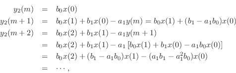
An example multi-input, multi-output (MIMO) digital filter is
![$\displaystyle \left[\begin{array}{c} y_1(n) \\ [2pt] y_2(n) \end{array}\right] ...
...y}\right]\left[\begin{array}{c} x_1(n-1) \\ [2pt] x_2(n-1) \end{array}\right],
$](http://www.dsprelated.com/josimages_new/filters/img426.png)
The simplest nonlinear digital filter is
Another nonlinear filter example is the
median smoother of order ![]() which assigns the middle value of
which assigns the middle value of
![]() input samples centered about time
input samples centered about time ![]() to the output at time
to the output at time ![]() .
It is useful for ``outlier'' elimination. For example, it will reject
isolated noise spikes, and preserve steps.
.
It is useful for ``outlier'' elimination. For example, it will reject
isolated noise spikes, and preserve steps.
An example of a linear time-varying filter is
These examples provide a kind of ``bottom up'' look at some of the major types of digital filters. We will now take a ``top down'' approach and characterize all linear, time-invariant filters mathematically. This characterization will enable us to specify frequency-domain analysis tools that work for any LTI digital filter.
Linear Filters
In everyday terms, the fact that a filter is linear means simply that
the following two properties hold:
Scaling:
The amplitude of the output is proportional to the amplitude of the input (the scaling property).
Superposition:
When two signals are added together and fed to the filter, the filter output is the same as if one had put each signal through the filter separately and then added the outputs (the superposition property).
While the implications of linearity are far-reaching, the mathematical definition is simple. Let us represent the general linear (but possibly time-varying) filter as a signal operator:
where
Definition. A filter
![]() is said to be
linear
if for any pair of signals
is said to be
linear
if for any pair of signals
![]() and for all
constant gains
and for all
constant gains ![]() , we have the following relation for each
sample time
, we have the following relation for each
sample time
![]() :
:
where
The scaling property of linear systems states that scaling the input of a linear system (multiplying it by a constant gain factor) scales the output by the same factor. The superposition property of linear systems states that the response of a linear system to a sum of signals is the sum of the responses to each individual input signal. Another view is that the individual signals which have been summed at the input are processed independently inside the filter--they superimpose and do not interact. (The addition of two signals, sample by sample, is like converting stereo to mono by mixing the two channels together equally.)
Another example of a linear signal medium is the earth's atmosphere. When two sounds are in the air at once, the air pressure fluctuations that convey them simply add (unless they are extremely loud). Since any finite continuous signal can be represented as a sum (i.e., superposition) of sinusoids, we can predict the filter response to any input signal just by knowing the response for all sinusoids. Without superposition, we have no such general description and it may be impossible to do any better than to catalog the filter output for each possible input.
Linear operators distribute over linear combinations, i.e.,
Real Linear Filtering of Complex Signals
When a filter
![]() is a linear filter (but not necessarily
time-invariant), and its input is a complex signal
is a linear filter (but not necessarily
time-invariant), and its input is a complex signal
![]() ,
then, by linearity,
,
then, by linearity,
Appendix H presents a linear-algebraic view of linear filters that can be useful in certain applications.
Time-Invariant Filters
In plain terms, a time-invariant
filter (or shift-invariant
filter) is one which performs the
same operation at all times. It is awkward to express this
mathematically by restrictions on Eq.![]() (4.2) because of the use of
(4.2) because of the use of
![]() as the symbol for the filter input. What we want to say is
that if the input signal is delayed (shifted) by, say,
as the symbol for the filter input. What we want to say is
that if the input signal is delayed (shifted) by, say, ![]() samples,
then the output waveform is simply delayed by
samples,
then the output waveform is simply delayed by ![]() samples and
unchanged otherwise. Thus
samples and
unchanged otherwise. Thus ![]() , the output waveform from a
time-invariant filter, merely shifts forward or backward in
time as the input waveform
, the output waveform from a
time-invariant filter, merely shifts forward or backward in
time as the input waveform ![]() is shifted forward or backward
in time.
is shifted forward or backward
in time.
Definition. A digital filter
![]() is said to be
time-invariant
if, for every input signal
is said to be
time-invariant
if, for every input signal ![]() , we have
, we have
where the
Showing Linearity and Time Invariance, or Not
The filter
![]() is nonlinear and time invariant. The
scaling property of linearity clearly fails since, scaling
is nonlinear and time invariant. The
scaling property of linearity clearly fails since, scaling ![]() by
by
![]() gives the output signal
gives the output signal
![]() , while
, while
![]() . The filter is time invariant, however, because delaying
. The filter is time invariant, however, because delaying ![]() by
by ![]() samples gives
samples gives ![]() which is the same as
which is the same as ![]() .
.
The filter
![]() is linear and time varying.
We can show linearity by setting the input to a linear combination of
two signals
is linear and time varying.
We can show linearity by setting the input to a linear combination of
two signals
![]() , where
, where ![]() and
and
![]() are constants:
are constants:
![\begin{eqnarray*}
n [\alpha x_1(n) + \beta x_2(n)] &+& [\alpha x_1(n-1) + \beta ...
... [n x_2(n) + x_2(n-1)]\\
&\isdef & \alpha y_1(n) + \beta y_2(n)
\end{eqnarray*}](http://www.dsprelated.com/josimages_new/filters/img469.png)
Thus, scaling and superposition are verified. The filter is
time-varying, however, since the time-shifted output is
![]() which is not the same as the filter applied
to a time-shifted input (
which is not the same as the filter applied
to a time-shifted input (
![]() ). Note that in
applying the time-invariance test, we time-shift the input signal
only, not the coefficients.
). Note that in
applying the time-invariance test, we time-shift the input signal
only, not the coefficients.
The filter ![]() , where
, where ![]() is any constant, is nonlinear
and time-invariant, in general. The condition for time invariance is
satisfied (in a degenerate way) because a constant signal equals all
shifts of itself. The constant filter is technically linear,
however, for
is any constant, is nonlinear
and time-invariant, in general. The condition for time invariance is
satisfied (in a degenerate way) because a constant signal equals all
shifts of itself. The constant filter is technically linear,
however, for ![]() , since
, since
![]() , even though the input
signal has no effect on the output signal at all.
, even though the input
signal has no effect on the output signal at all.
Any filter of the form
![]() is linear and
time-invariant. This is a special case of a sliding linear
combination (also called a running weighted sum, or
moving average when
is linear and
time-invariant. This is a special case of a sliding linear
combination (also called a running weighted sum, or
moving average when
![]() ).
All sliding linear combinations are linear,
and they are time-invariant as well when the coefficients (
).
All sliding linear combinations are linear,
and they are time-invariant as well when the coefficients (
![]() ) are constant with respect to time.
) are constant with respect to time.
Sliding linear combinations may also include past output samples as well (feedback terms). A simple example is any filter of the form
Since linear combinations of linear combinations are linear combinations, we can use induction to show linearity and time invariance of a constant sliding linear combination including feedback terms. In the case of this example, we have, for an input signal

If the input signal is now replaced by
![]() ,
which is
,
which is ![]() delayed by
delayed by ![]() samples, then the
output
samples, then the
output ![]() is
is ![]() for
for ![]() , followed by
, followed by
or
![]() for all
for all ![]() and
and ![]() . This establishes
that each output sample from the filter of Eq.
. This establishes
that each output sample from the filter of Eq.![]() (4.7) can be expressed
as a time-invariant linear combination of present and past samples.
(4.7) can be expressed
as a time-invariant linear combination of present and past samples.
Nonlinear Filter Example:
Dynamic Range Compression
A simple practical example of a nonlinear filtering operation is dynamic range compression, such as occurs in Dolby or DBX noise reduction when recording to magnetic tape (which, believe it or not, still happens once in a while). The purpose of dynamic range compression is to map the natural dynamic range of a signal to a smaller range. For example, audio signals can easily span a range of 100 dB or more, while magnetic tape has a linear range on the order of only 55 dB. It is therefore important to compress the dynamic range when making analog recordings to magnetic tape. Compressing the dynamic range of a signal for recording and then expanding it on playback may be called companding (compression/expansion).
Recording engineers often compress the dynamic range of individual tracks to intentionally ``flatten'' their audio dynamic range for greater musical uniformity. Compression is also often applied to a final mix.
Another type of dynamic-range compressor is called a limiter, which is used in recording studios to ``soft limit'' a signal when it begins to exceed the available dynamic range. A limiter may be implemented as a very high compression ratio above some amplitude threshold. This replaces ``hard clipping'' by ``soft limiting,'' which sounds less harsh and may even go unnoticed if there were no indicator.
The preceding examples can be modeled as a variable gain that automatically ``turns up the volume'' (increases the gain) when the signal level is low, and turns it down when the level is high. The signal level is normally measured over a short time interval that includes at least one period of the lowest frequency allowed, and typically several periods of any pitched signal present. The gain normally reacts faster to attacks than to decays in audio compressors.
Why Dynamic Range Compression is Nonlinear
We can model dynamic range compression as a level-dependent
gain. Multiplying a signal by a constant gain (``volume control''),
on the other hand, is a linear operation. Let's check that the
scaling and superposition properties of linear systems are satisfied
by a constant gain: For any signals ![]() , and for any constants
, and for any constants
![]() , we must have
, we must have
Dynamic range compression can also be seen as a time-varying
gain factor, so one might be tempted to classify it as a linear,
time-varying filter. However, this would be incorrect because the
gain ![]() , which multiplies the input, depends on the input
signal
, which multiplies the input, depends on the input
signal ![]() . This happens because the compressor must estimate the
current signal level in order to normalize it. Dynamic range
compression can be expressed symbolically as a filter of the form
. This happens because the compressor must estimate the
current signal level in order to normalize it. Dynamic range
compression can be expressed symbolically as a filter of the form
In general, any signal operation that includes a multiplication in which both multiplicands depend on the input signal can be shown to be nonlinear.
A Musical Time-Varying Filter Example
Note, however, that a gain ![]() may vary with time independently
of
may vary with time independently
of ![]() to yield a linear time-varying filter. In this case,
linearity may be demonstrated by verifying
to yield a linear time-varying filter. In this case,
linearity may be demonstrated by verifying
Analysis of Nonlinear Filters
There is no general theory of nonlinear systems. A nonlinear system with memory can be quite surprising. In particular, it can emit any output signal in response to any input signal. For example, it could replace all music by Beethoven with something by Mozart, etc. That said, many subclasses of nonlinear filters can be successfully analyzed:
- A nonlinear, memoryless, time-invariant ``black box'' can be ``mapped
out'' by measuring its response to a scaled impulse
 at each amplitude
  , where
  denotes the impulse
signal (
denotes the impulse
signal (
![$ [1,0,0,\ldots]$](http://www.dsprelated.com/josimages_new/filters/img499.png) ).
).
- A memoryless nonlinearity followed by an LTI filter can similarly be characterized by a stack of impulse-responses indexed by amplitude (look up dynamic convolution on the Web).
One often-used tool for nonlinear systems analysis is Volterra series [4]. A Volterra series expansion represents a nonlinear system as a sum of iterated convolutions:
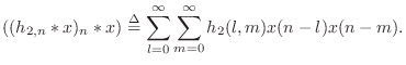
In the special case for which the Volterra expansion reduces to
Conclusions
This chapter has discussed the concepts of linearity and time-invariance in some detail, with various examples considered. In the rest of this book, all filters discussed will be linear and (at least approximately) time-invariant. For brevity, these will be referred to as LTI filters.
Linearity and Time-Invariance Problems
See http://ccrma.stanford.edu/~jos/filtersp/Linearity_Time_Invariance_Problems.html
Next Section:
Time Domain Digital Filter Representations
Previous Section:
Analysis of a Digital Comb Filter


