


Moving Mass
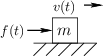
Figure D.1 depicts a free mass driven by an external force along
an ideal frictionless surface in one dimension. Figure D.2
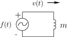
shows the electrical equivalent circuit for this scenario in
which the external force is represented by a voltage source emitting
![]() volts, and the mass is modeled by an inductor
having the value
volts, and the mass is modeled by an inductor
having the value ![]() Henrys.
Henrys.
From Newton's second law of motion ``![]() '', we have
'', we have
![\begin{eqnarray*}
F(s) &=& m\,{\cal L}_s\{{\ddot x}\}\\
&=& m\left[\,s {\cal L...
...right\}\\
&=& m\left[s^2\,X(s) - s\,x(0) - {\dot x}(0)\right].
\end{eqnarray*}](http://www.dsprelated.com/josimages_new/filters/img1738.png)
Thus, given
 Laplace transform of the driving force
  ,
,
 initial mass position, and
-
 initial mass velocity,
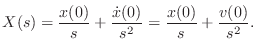
If the applied external force ![]() is zero, then, by linearity of
the Laplace transform, so is
is zero, then, by linearity of
the Laplace transform, so is ![]() , and we readily obtain
, and we readily obtain
![$\displaystyle u(t)\isdef \left\{\begin{array}{ll}
0, & t<0 \\ [5pt]
1, & t\ge 0 \\
\end{array}\right.,
$](http://www.dsprelated.com/josimages_new/filters/img1745.png)
To summarize, this simple example illustrated use the Laplace transform to solve for the motion of a simple physical system (an ideal mass) in response to initial conditions (no external driving forces). The system was described by a differential equation which was converted to an algebraic equation by the Laplace transform.
Next Section:
Mass-Spring Oscillator Analysis
Previous Section:
Differentiation


