


Mass-Spring Oscillator Analysis
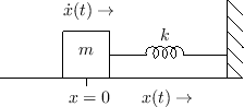
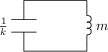
Consider now the mass-spring oscillator depicted physically in Fig.D.3, and in equivalent-circuit form in Fig.D.4.
 |
By Newton's second law of motion, the force ![]() applied to a mass
equals its mass times its acceleration:
applied to a mass
equals its mass times its acceleration:
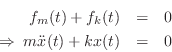
We have thus derived a second-order differential equation governing
the motion of the mass and spring. (Note that ![]() in
Fig.D.3 is both the position of the mass and compression
of the spring at time
in
Fig.D.3 is both the position of the mass and compression
of the spring at time ![]() .)
.)
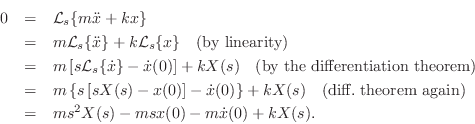
Taking the Laplace transform of both sides of this differential equation gives
To simplify notation, denote the initial position and velocity by
![]() and
and
![]() , respectively. Solving for
, respectively. Solving for ![]() gives
gives
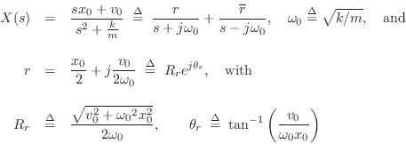
denoting the modulus and angle of the pole residue ![]() , respectively.
From §D.1, the inverse Laplace transform of
, respectively.
From §D.1, the inverse Laplace transform of ![]() is
is
![]() , where
, where ![]() is the Heaviside unit step function at time 0.
Then by linearity, the solution for
the motion of the mass is
is the Heaviside unit step function at time 0.
Then by linearity, the solution for
the motion of the mass is
![\begin{eqnarray*}
x(t) &=& re^{-j{\omega_0}t} + \overline{r}e^{j{\omega_0}t}
= ...
...ga_0}t - \tan^{-1}\left(\frac{v_0}{{\omega_0}x_0}\right)\right].
\end{eqnarray*}](http://www.dsprelated.com/josimages_new/filters/img1771.png)
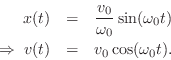
If the initial velocity is zero (![]() ), the above formula
reduces to
), the above formula
reduces to
![]() and the mass simply oscillates sinusoidally at frequency
and the mass simply oscillates sinusoidally at frequency
![]() , starting from its initial position
, starting from its initial position ![]() .
If instead the initial position is
.
If instead the initial position is ![]() , we obtain
, we obtain
Mechanical Equivalent of a Capacitor is a Spring
The mechanical analog of a capacitor is the compliance of a
spring. The voltage ![]() across a capacitor
across a capacitor ![]() corresponds to the
force
corresponds to the
force ![]() used to displace a spring. The charge
used to displace a spring. The charge ![]() stored in
the capacitor corresponds to the displacement
stored in
the capacitor corresponds to the displacement ![]() of the spring.
Thus, Eq.
of the spring.
Thus, Eq.![]() (E.2) corresponds to Hooke's law for ideal springs:
(E.2) corresponds to Hooke's law for ideal springs:
Mechanical Equivalent of an Inductor is a Mass
The mechanical analog of an inductor is a mass. The voltage
![]() across an inductor
across an inductor ![]() corresponds to the force
corresponds to the force ![]() used to
accelerate a mass
used to
accelerate a mass ![]() . The current
. The current ![]() through in the inductor
corresponds to the velocity
through in the inductor
corresponds to the velocity
![]() of the mass. Thus,
Eq.
of the mass. Thus,
Eq.![]() (E.4) corresponds to Newton's second law for an ideal mass:
(E.4) corresponds to Newton's second law for an ideal mass:
From the defining equation ![]() for an inductor [Eq.
for an inductor [Eq.![]() (E.3)], we
see that the stored magnetic flux in an inductor is analogous to mass
times velocity, or momentum. In other words, magnetic flux may
be regarded as electric-charge momentum.
(E.3)], we
see that the stored magnetic flux in an inductor is analogous to mass
times velocity, or momentum. In other words, magnetic flux may
be regarded as electric-charge momentum.
Next Section:
Driving Point Impedance
Previous Section:
Moving Mass


