


So What's Up with Repeated Poles?
In the previous section, we found that repeated poles give rise to polynomial amplitude-envelopes multiplying the exponential decay due to the pole. On the other hand, two different poles can only yield a convolution (or sum) of two different exponential decays, with no polynomial envelope allowed. This is true no matter how closely the poles come together; the polynomial envelope can occur only when the poles merge exactly. This might violate one's intuitive expectation of a continuous change when passing from two closely spaced poles to a repeated pole.
To study this phenomenon further, consider the convolution of two
one-pole impulse-responses
![]() and
and
![]() :
:
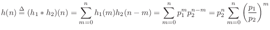
The finite limits on the summation result from the fact that both
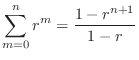
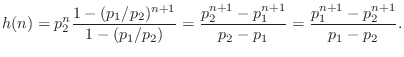
Going back to Eq.![]() (6.14), we have
(6.14), we have
 |
(7.15) |
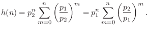
Setting
| (7.16) |
which is the first-order polynomial amplitude-envelope case for a repeated pole. We can see that the transition from ``two convolved exponentials'' to ``single exponential with a polynomial amplitude envelope'' is perfectly continuous, as we would expect.
We also see that the polynomial amplitude-envelopes fundamentally
arise from iterated convolutions. This corresponds to the
repeated poles being arranged in series, rather than in
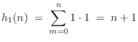
parallel. The simplest case is when the repeated pole is at ![]() , in
which case its impulse response is a constant:
, in
which case its impulse response is a constant:

Next Section:
Example 2
Previous Section:
Impulse Response of Repeated Poles


