FM Spectra
Using the expansion in Eq. (4.7), it is now easy to determine
the spectrum of sinusoidal FM. Eliminating scaling and
phase offsets for simplicity in Eq.(4.5) yields
(4.7), it is now easy to determine
the spectrum of sinusoidal FM. Eliminating scaling and
phase offsets for simplicity in Eq.(4.5) yields
![$\displaystyle x(t) = \cos[\omega_c t + \beta\sin(\omega_m t)], \protect$](http://www.dsprelated.com/josimages_new/mdft/img538.png) |
(4.8) |
where we have changed the modulator amplitude

to the more
traditional symbol

, called the
FM index in FM sound
synthesis contexts. Using
phasor analysis (where
phasors
are defined below in §
4.3.11),
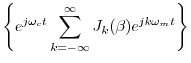
4.11i.e., expressing a real-valued FM
signal as the real part of a more
analytically tractable complex-valued FM signal, we obtain
where we used the fact that

is real when
is real.
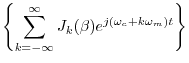
We can now see clearly that the sinusoidal FM spectrum consists of an
infinite number of side-bands about the carrier frequency

(when

). The side bands occur at multiples of the
modulating frequency

away from the carrier frequency
.
Next Section: PhasorPrevious Section: Bessel Functions


![$\displaystyle \sum_{k=-\infty}^\infty J_k(\beta) \cos[(\omega_c+k\omega_m) t]$](http://www.dsprelated.com/josimages_new/mdft/img545.png)


