


Gram-Schmidt Orthogonalization
Recall from the end of §5.10 above that an
orthonormal set of vectors is a set of unit-length
vectors that are mutually orthogonal. In other words,
orthonormal vector set is just an orthogonal vector set in which each
vector ![]() has been normalized to unit length
has been normalized to unit length
![]() .
.
Theorem: Given a set of ![]() linearly independent vectors
linearly independent vectors
![]() from
from ![]() , we can construct an
orthonormal set
, we can construct an
orthonormal set
![]() which are linear
combinations of the original set and which span the same space.
which are linear
combinations of the original set and which span the same space.
Proof: We prove the theorem by constructing the desired orthonormal
set
![]() sequentially from the original set
sequentially from the original set ![]() .
This procedure is known as Gram-Schmidt orthogonalization.
.
This procedure is known as Gram-Schmidt orthogonalization.
First, note that
![]() for all
for all ![]() , since
, since
![]() is
linearly dependent on every vector. Therefore,
is
linearly dependent on every vector. Therefore,
![]() .
.
- Set
 .
.
- Define
 as
as  minus the projection of
onto
minus the projection of
onto
 :
The vector
:
The vector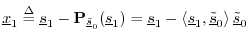 is orthogonal to
by construction. (We
subtracted out the part of that wasn't orthogonal to
.) Also, since and
is orthogonal to
by construction. (We
subtracted out the part of that wasn't orthogonal to
.) Also, since and  are linearly independent,
we have
are linearly independent,
we have
 .
.
- Set
 (i.e., normalize the result
of the preceding step).
(i.e., normalize the result
of the preceding step).
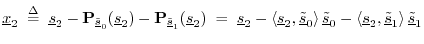
- Define
 as
as  minus the projection of
onto
and
minus the projection of
onto
and
 :
:
- Normalize:
 .
.
- Continue this process until
 has been defined.
The Gram-Schmidt orthogonalization procedure will construct an
orthonormal basis from any set of ![]() linearly independent vectors.
Obviously, by skipping the normalization step, we could also form
simply an orthogonal basis. The key ingredient of this procedure is
that each new basis vector is obtained by subtracting out the
projection of the next linearly independent vector onto the vectors
accepted so far into the set. We may say that each new linearly
independent vector
linearly independent vectors.
Obviously, by skipping the normalization step, we could also form
simply an orthogonal basis. The key ingredient of this procedure is
that each new basis vector is obtained by subtracting out the
projection of the next linearly independent vector onto the vectors
accepted so far into the set. We may say that each new linearly
independent vector ![]() is projected onto the subspace
spanned by the vectors
is projected onto the subspace
spanned by the vectors
![]() , and any nonzero
projection in that subspace is subtracted out of
, and any nonzero
projection in that subspace is subtracted out of ![]() to make the
new vector orthogonal to the entire subspace. In other words, we
retain only that portion of each new vector
to make the
new vector orthogonal to the entire subspace. In other words, we
retain only that portion of each new vector ![]() which ``points
along'' a new dimension. The first direction is arbitrary and is
determined by whatever vector we choose first (
which ``points
along'' a new dimension. The first direction is arbitrary and is
determined by whatever vector we choose first (![]() here). The
next vector is forced to be orthogonal to the first. The second is
forced to be orthogonal to the first two (and thus to the 2D subspace
spanned by them), and so on.
here). The
next vector is forced to be orthogonal to the first. The second is
forced to be orthogonal to the first two (and thus to the 2D subspace
spanned by them), and so on.
This chapter can be considered an introduction to some important concepts of linear algebra. The student is invited to pursue further reading in any textbook on linear algebra, such as [47].5.13
Matlab/Octave examples related to this chapter appear in Appendix I.
Next Section:
Nth Roots of Unity
Previous Section:
Signal/Vector Reconstruction from Projections


