


The Inner Product
The inner product (or ``dot product'', or ``scalar product'')
is an operation on two vectors which produces a scalar. Defining an
inner product for a Banach space specializes it to a Hilbert
space (or ``inner product space''). There are many examples of
Hilbert spaces, but we will only need
![]() for this
book (complex length
for this
book (complex length ![]() vectors, and complex scalars).
vectors, and complex scalars).
The inner product between (complex) ![]() -vectors
-vectors
![]() and
and
![]() is
defined by5.9
is
defined by5.9
The complex conjugation of the second vector is done in order that a norm will be induced by the inner product:5.10
Note that the inner product takes
![]() to
to ![]() . That
is, two length
. That
is, two length ![]() complex vectors are mapped to a complex scalar.
complex vectors are mapped to a complex scalar.
Linearity of the Inner Product
Any function
![]() of a vector
of a vector
![]() (which we may call an
operator on
(which we may call an
operator on ![]() ) is said to be linear if for all
) is said to be linear if for all
![]() and
and
![]() , and for all scalars
, and for all scalars ![]() and
and ![]() in
in
![]() ,
,
- additivity:
- homogeneity:
The inner product
![]() is linear in its first argument, i.e.,
for all
is linear in its first argument, i.e.,
for all
![]() , and for all
, and for all
![]() ,
,
The inner product is also additive in its second argument, i.e.,
The inner product is strictly linear in its second argument with
respect to real scalars ![]() and
and ![]() :
:
Since the inner product is linear in both of its arguments for real scalars, it may be called a bilinear operator in that context.
Norm Induced by the Inner Product
We may define a norm on
![]() using the inner product:
using the inner product:
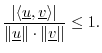
Cauchy-Schwarz Inequality
The Cauchy-Schwarz Inequality (or ``Schwarz Inequality'')
states that for all
![]() and
and
![]() , we have
, we have
We can quickly show this for real vectors
![]() ,
,
![]() , as
follows: If either
, as
follows: If either
![]() or
or
![]() is zero, the inequality holds (as
equality). Assuming both are nonzero, let's scale them to unit-length
by defining the normalized vectors
is zero, the inequality holds (as
equality). Assuming both are nonzero, let's scale them to unit-length
by defining the normalized vectors
![]() ,
,
![]() , which are
unit-length vectors lying on the ``unit ball'' in
, which are
unit-length vectors lying on the ``unit ball'' in ![]() (a hypersphere
of radius
(a hypersphere
of radius ![]() ). We have
). We have
which implies
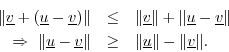
Triangle Inequality
The triangle inequality states that the length of any side of a
triangle is less than or equal to the sum of the lengths of the other two
sides, with equality occurring only when the triangle degenerates to a
line. In ![]() , this becomes
, this becomes
Triangle Difference Inequality
A useful variation on the triangle inequality is that the length of any side of a triangle is greater than the absolute difference of the lengths of the other two sides:
Proof: By the triangle inequality,
Interchanging
![]() and
and
![]() establishes the absolute value on the
right-hand side.
establishes the absolute value on the
right-hand side.
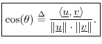
Vector Cosine
The Cauchy-Schwarz Inequality can be written
Orthogonality
The vectors (signals) ![]() and
and
![]() 5.11are said to be orthogonal if
5.11are said to be orthogonal if
![]() , denoted
, denoted ![]() .
That is to say
.
That is to say
Note that if ![]() and
and ![]() are real and orthogonal, the cosine of the angle
between them is zero. In plane geometry (
are real and orthogonal, the cosine of the angle
between them is zero. In plane geometry (![]() ), the angle between two
perpendicular lines is
), the angle between two
perpendicular lines is ![]() , and
, and
![]() , as expected. More
generally, orthogonality corresponds to the fact that two vectors in
, as expected. More
generally, orthogonality corresponds to the fact that two vectors in
![]() -space intersect at a right angle and are thus perpendicular
geometrically.
-space intersect at a right angle and are thus perpendicular
geometrically.
Example (![]() ):
):
Let ![]() and
and ![]() , as shown in Fig.5.8.
, as shown in Fig.5.8.
![\includegraphics[scale=0.7]{eps/ip}](http://www.dsprelated.com/josimages_new/mdft/img856.png)
The inner product is
![]() .
This shows that the vectors are orthogonal. As marked in the figure,
the lines intersect at a right angle and are therefore perpendicular.
.
This shows that the vectors are orthogonal. As marked in the figure,
the lines intersect at a right angle and are therefore perpendicular.
The Pythagorean Theorem in N-Space
In 2D, the Pythagorean Theorem says that when ![]() and
and ![]() are
orthogonal, as in Fig.5.8, (i.e., when the vectors
are
orthogonal, as in Fig.5.8, (i.e., when the vectors ![]() and
and ![]() intersect at a right angle), then we have
intersect at a right angle), then we have
This relationship generalizes to
If
Note that the converse is not true in ![]() . That is,
. That is,
![]() does not imply
does not imply
![]() in
in ![]() . For a counterexample, consider
. For a counterexample, consider ![]() ,
,
![]() , in which case
, in which case
For real vectors
![]() , the Pythagorean theorem Eq.
, the Pythagorean theorem Eq.![]() (5.1)
holds if and only if the vectors are orthogonal. To see this, note
that, from Eq.
(5.1)
holds if and only if the vectors are orthogonal. To see this, note
that, from Eq.![]() (5.2), when the Pythagorean theorem holds, either
(5.2), when the Pythagorean theorem holds, either
![]() or
or ![]() is zero, or
is zero, or
![]() is zero or purely imaginary,
by property 1 of norms (see §5.8.2). If the inner product
cannot be imaginary, it must be zero.
is zero or purely imaginary,
by property 1 of norms (see §5.8.2). If the inner product
cannot be imaginary, it must be zero.
Note that we also have an alternate version of the Pythagorean theorem:
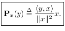
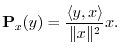
Projection
The orthogonal projection (or simply ``projection'') of
![]() onto
onto
![]() is defined by
is defined by
Motivation: The basic idea of orthogonal projection of ![]() onto
onto
![]() is to ``drop a perpendicular'' from
is to ``drop a perpendicular'' from ![]() onto
onto ![]() to define a new
vector along
to define a new
vector along ![]() which we call the ``projection'' of
which we call the ``projection'' of ![]() onto
onto ![]() .
This is illustrated for
.
This is illustrated for ![]() in Fig.5.9 for
in Fig.5.9 for ![]() and
and
![]() , in which case
, in which case
![$\displaystyle {\bf P}_{x}(y) \isdef \frac{\left<y,x\right>}{\Vert x\Vert^2} x
...
...{1})}{4^2+1^2} x
= \frac{11}{17} x= \left[\frac{44}{17},\frac{11}{17}\right].
$](http://www.dsprelated.com/josimages_new/mdft/img880.png)
![\includegraphics[scale=0.7]{eps/proj}](http://www.dsprelated.com/josimages_new/mdft/img881.png)
Derivation: (1) Since any projection onto ![]() must lie along the
line collinear with
must lie along the
line collinear with ![]() , write the projection as
, write the projection as
![]() . (2) Since by definition the projection error
. (2) Since by definition the projection error
![]() is orthogonal to
is orthogonal to ![]() , we must have
, we must have
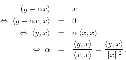
Thus,
See §I.3.3 for illustration of orthogonal projection in matlab.
Next Section:
Signal Reconstruction from Projections
Previous Section:
Signal Metrics


