


Projection
As discussed in §5.9.9,
the orthogonal projection of
![]() onto
onto
![]() is defined by
is defined by
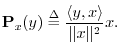
yx = (x' * y) * (x' * x)^(-1) * xMore generally, a length-N column-vector y can be projected onto the
yX = X * (X' * X)^(-1) * X' * yOrthogonal projection, like any finite-dimensional linear operator, can be represented by a matrix. In this case, the
PX = X * (X' * X)^(-1) * X'is called the projection matrix.I.2Subspace projection is an example in which the power of matrix linear algebra notation is evident.
Projection Example 1
>> X = [[1;2;3],[1;0;1]]
X =

   1   1
   2   0
   3   1

>> PX = X * (X' * X)^(-1) * X'
PX =

   0.66667  -0.33333   0.33333
  -0.33333   0.66667   0.33333
   0.33333   0.33333   0.66667

>> y = [2;4;6]
y =

   2
   4
   6

>> yX = PX * y
yX =

   2.0000
   4.0000
   6.0000
Since y in this example already lies in the column-space of X, orthogonal projection onto that space has no effect.
Projection Example 2
Let X and PX be defined as Example 1, but now let
>> y = [1;-1;1]
y =

   1
  -1
   1

>> yX = PX * y
yX =

   1.33333
  -0.66667
   0.66667

>> yX' * (y-yX)
ans = -7.0316e-16

>> eps
ans =  2.2204e-16
In the last step above, we verified that the projection yX is
orthogonal to the ``projection error'' y-yX, at least to
machine precision. The eps variable holds ``machine
epsilon'' which is the numerical distance
between ![]() and the next representable number in double-precision
floating point.
and the next representable number in double-precision
floating point.
Next Section:
Orthogonal Basis Computation
Previous Section:
Vector Cosine


