


Number Systems for Digital Audio
This appendix discusses number formats used in digital audio. They
are divided into ``linear'' and ``logarithmic.'' Linear number
systems include binary integer fixed-point, fractional fixed-point,
one's complement, and two's complement fixed-point. The ![]() -law
format is a popular hybrid between linear and logarithmic amplitude
encoding. Floating-point combines a linear mantissa with a logarithmic
``exponent,'' and logarithmic fixed-point can be viewed as a special
case of floating-point in which there is no mantissa. This appendix
does not cover audio coding methods such as MPEG (MP3)
[5,7,50,6]
or Linear Predictive Coding (LPC) [11,40,41].
-law
format is a popular hybrid between linear and logarithmic amplitude
encoding. Floating-point combines a linear mantissa with a logarithmic
``exponent,'' and logarithmic fixed-point can be viewed as a special
case of floating-point in which there is no mantissa. This appendix
does not cover audio coding methods such as MPEG (MP3)
[5,7,50,6]
or Linear Predictive Coding (LPC) [11,40,41].
Linear Number Systems
Linear number systems are used in digital audio gear such as compact disks and digital audio tapes. As such, they represent the ``high end'' of digital audio formats, when a sufficiently large sampling rate (e.g., above 40 kHz) and number of bits per word (e.g., 20), are used.
Pulse Code Modulation (PCM)
The ``standard'' number format for sampled audio signals is officially called Pulse Code Modulation (PCM). This term simply means that each signal sample is interpreted as a ``pulse'' (e.g., a voltage or current pulse) at a particular amplitude which is binary encoded, typically in two's complement binary fixed-point format (discussed below). When someone says they are giving you a soundfile in ``raw binary format'', they pretty much always mean (nowadays) 16-bit, two's-complement PCM data. Most mainstream computer soundfile formats consist of a ``header'' (containing the length, etc.) followed by 16-bit two's-complement PCM.
You can normally convert a soundfile from one computer's format to another by stripping off its header and prepending the header for the new machine (or simply treating it as raw binary format on the destination computer). The UNIX ``cat'' command can be used for this, as can the Emacs text editor (which handles binary data just fine). The only issue usually is whether the bytes have to be swapped (an issue discussed further below).
Binary Integer Fixed-Point Numbers
Most computer languages nowadays only offer two kinds of numbers, floating-point and integer fixed-point. On present-day computers, all numbers are encoded using binary digits (called ``bits'') which are either 1 or 0.G.1 In C, C++, and Java, floating-point variables are declared as float (32 bits) or double (64 bits), while integer fixed-point variables are declared as short int (typically 16 bits and never less), long int (typically 32 bits and never less), or simply int (typically the same as a long int, but sometimes between short and long). For an 8-bit integer, one can use the char data type (8 bits).
Since C was designed to accommodate a wide range of hardware, including old mini-computers, some latitude was historically allowed in the choice of these bit-lengths. The sizeof operator is officially the ``right way'' for a C program to determine the number of bytes in various data types at run-time, e.g., sizeof(long). (The word int can be omitted after short or long.) Nowadays, however, shorts are always 16 bits (at least on all the major platforms), ints are 32 bits, and longs are typically 32 bits on 32-bit computers and 64 bits on 64-bit computers (although some C/C++ compilers use long long int to declare 64-bit ints). Table G.1 gives the lengths currently used by GNU C/C++ compilers (usually called ``gcc'' or ``cc'') on 64-bit processors.G.2
Java, which is designed to be platform independent, defines a long int as equivalent in precision to 64 bits, an int
as 32 bits, a short int as 16 bits, and additionally a byte
int as an 8-bit int. Similarly, the ``Structured Audio Orchestra
Language''
(SAOL)
(pronounced ``sail'')--the sound-synthesis component of the new
MPEG-4 audio compression standard--requires only that the underlying number
system be at least as accurate as 32-bit floats. All ints
discussed thus far are signed integer formats. C and C++ also
support unsigned versions of all int types, and they range
from 0 to ![]() instead of
instead of ![]() to
to ![]() , where
, where ![]() is the number of bits. Finally, an unsigned char is often used for
integers that only range between 0 and 255.
is the number of bits. Finally, an unsigned char is often used for
integers that only range between 0 and 255.
One's Complement Fixed-Point Format
One's Complement is a particular assignment of bit patterns to numbers. For example, in the case of 3-bit binary numbers, we have the assignments shown in Table G.2.
|
In general, ![]() -bit numbers are assigned to binary counter values in
the ``obvious way'' as integers from 0 to
-bit numbers are assigned to binary counter values in
the ``obvious way'' as integers from 0 to ![]() , and then the
negative numbers are assigned in reverse order, as shown in the
example.
, and then the
negative numbers are assigned in reverse order, as shown in the
example.
The term ``one's complement'' refers to the fact that negating a number in this format is accomplished by simply complementing the bit pattern (inverting each bit).
Note that there are two representations for zero (all 0s and all 1s). This is inconvenient when testing if a number is equal to zero. For this reason, one's complement is generally not used.
Two's Complement Fixed-Point Format
In two's complement, numbers are negated by complementing the
bit pattern and adding 1, with overflow ignored. From 0 to
![]() , positive numbers are assigned to binary values exactly as
in one's complement. The remaining assignments (for the negative
numbers) can be carried out using the two's complement negation rule.
Regenerating the
, positive numbers are assigned to binary values exactly as
in one's complement. The remaining assignments (for the negative
numbers) can be carried out using the two's complement negation rule.
Regenerating the ![]() example in this way gives Table G.3.
example in this way gives Table G.3.
|
Note that according to our negation rule,
![]() . Logically,
what has happened is that the result has ``overflowed'' and ``wrapped
around'' back to itself. Note that
. Logically,
what has happened is that the result has ``overflowed'' and ``wrapped
around'' back to itself. Note that ![]() also. In other words, if
you compute 4 somehow, since there is no bit-pattern assigned to 4,
you get -4, because -4 is assigned the bit pattern that would be
assigned to 4 if
also. In other words, if
you compute 4 somehow, since there is no bit-pattern assigned to 4,
you get -4, because -4 is assigned the bit pattern that would be
assigned to 4 if ![]() were larger. Note that numerical overflows
naturally result in ``wrap around'' from positive to negative numbers
(or from negative numbers to positive numbers). Computers normally
``trap'' overflows as an ``exception.'' The exceptions are usually
handled by a software ``interrupt handler,'' and this can greatly slow
down the processing by the computer (one numerical calculation is
being replaced by a rather sizable program).
were larger. Note that numerical overflows
naturally result in ``wrap around'' from positive to negative numbers
(or from negative numbers to positive numbers). Computers normally
``trap'' overflows as an ``exception.'' The exceptions are usually
handled by a software ``interrupt handler,'' and this can greatly slow
down the processing by the computer (one numerical calculation is
being replaced by a rather sizable program).
Note that temporary overflows are ok in two's complement; that is, if
you add ![]() to
to ![]() to get
to get ![]() , adding
, adding ![]() to
to ![]() will give
will give ![]() again.
This is why two's complement is a nice choice: it can be thought of as
placing all the numbers on a ``ring,'' allowing temporary overflows of
intermediate results in a long string of additions and/or subtractions.
All that matters is that the final sum lie within the supported dynamic
range.
again.
This is why two's complement is a nice choice: it can be thought of as
placing all the numbers on a ``ring,'' allowing temporary overflows of
intermediate results in a long string of additions and/or subtractions.
All that matters is that the final sum lie within the supported dynamic
range.
Computers designed with signal processing in mind (such as so-called ``Digital Signal Processing (DSP) chips'') generally just do the best they can without generating exceptions. For example, overflows quietly ``saturate'' instead of ``wrapping around'' (the hardware simply replaces the overflow result with the maximum positive or negative number, as appropriate, and goes on). Since the programmer may wish to know that an overflow has occurred, the first occurrence may set an ``overflow indication'' bit which can be manually cleared. The overflow bit in this case just says an overflow happened sometime since it was last checked.
Two's-Complement, Integer Fixed-Point Numbers
Let ![]() denote the number of bits. Then the value of a two's
complement integer fixed-point number can be expressed in terms of its
bits
denote the number of bits. Then the value of a two's
complement integer fixed-point number can be expressed in terms of its
bits
![]() as
as
We visualize the binary word containing these bits as
The most-significant bit in the word, ![]() , can be interpreted as the
``sign bit''. If
, can be interpreted as the
``sign bit''. If ![]() is ``on'', the number is negative. If it is
``off'', the number is either zero or positive.
is ``on'', the number is negative. If it is
``off'', the number is either zero or positive.
The least-significant bit is ![]() . ``Turning on'' that bit adds 1 to
the number, and there are no fractions allowed.
. ``Turning on'' that bit adds 1 to
the number, and there are no fractions allowed.
The largest positive number is when all bits are on except ![]() , in
which case
, in
which case
![]() . The largest (in magnitude) negative number is
. The largest (in magnitude) negative number is
![]() , i.e.,
, i.e., ![]() and
and ![]() for all
for all ![]() . Table G.4 shows
some of the most common cases.
. Table G.4 shows
some of the most common cases.
|
Fractional Binary Fixed-Point Numbers
In ``DSP chips'' (microprocessors explicitly designed for digital signal processing applications), the most commonly used fixed-point format is fractional fixed point, also in two's complement.
Quite simply, fractional fixed-point numbers are obtained
from integer fixed-point numbers by dividing them by ![]() .
Thus, the only difference is a scaling of the assigned numbers.
In the
.
Thus, the only difference is a scaling of the assigned numbers.
In the ![]() case, we have the correspondences shown in Table G.5.
case, we have the correspondences shown in Table G.5.
|
How Many Bits are Enough for Digital Audio?
Armed with the above knowledge, we can visit the question ``how many
bits are enough'' for digital audio. Since the threshold of hearing
is around 0 db SPL, the ``threshold of pain'' is around 120 dB SPL,
and each bit in a linear PCM format is worth about
![]() dB of dynamic range, we find that we need
dB of dynamic range, we find that we need
![]() bits to
represent the full dynamic range of audio in a linear fixed-point
format. This is a simplistic analysis because it is not quite right
to equate the least-significant bit with the threshold of hearing;
instead, we would like to adjust the quantization noise floor
to just below the threshold of hearing. Since the threshold of
hearing is non-uniform, we would also prefer a shaped
quantization noise floor (a feat that can be accomplished using
filtered error feedbackG.3.) Nevertheless, the simplistic result gives an
answer similar to the more careful analysis, and 20 bits is a good number.
However, this still does not provide for
headroom needed in a digital recording scenario. We also need both
headroom and guard bits on the lower end when we plan to carry
out a lot of signal processing operations, especially digital
filtering. As an example, a 1024-point FFT (Fast Fourier Transform)
can give amplitudes 1024 times the input amplitude (such as in the
case of a constant ``dc'' input signal), thus requiring 10 headroom
bits. In general, 24 fixed-point bits are pretty reasonable to work
with, although you still have to scale very carefully, and 32 bits are
preferable.
bits to
represent the full dynamic range of audio in a linear fixed-point
format. This is a simplistic analysis because it is not quite right
to equate the least-significant bit with the threshold of hearing;
instead, we would like to adjust the quantization noise floor
to just below the threshold of hearing. Since the threshold of
hearing is non-uniform, we would also prefer a shaped
quantization noise floor (a feat that can be accomplished using
filtered error feedbackG.3.) Nevertheless, the simplistic result gives an
answer similar to the more careful analysis, and 20 bits is a good number.
However, this still does not provide for
headroom needed in a digital recording scenario. We also need both
headroom and guard bits on the lower end when we plan to carry
out a lot of signal processing operations, especially digital
filtering. As an example, a 1024-point FFT (Fast Fourier Transform)
can give amplitudes 1024 times the input amplitude (such as in the
case of a constant ``dc'' input signal), thus requiring 10 headroom
bits. In general, 24 fixed-point bits are pretty reasonable to work
with, although you still have to scale very carefully, and 32 bits are
preferable.
When Do We Have to Swap Bytes?
When moving a soundfile from one computer to another, such as from a ``PC'' to a ``Mac'' (Intel processor to Motorola processor), the bytes in each sound sample have to be swapped. This is because Motorola processors are big endian (bytes are numbered from most-significant to least-significant in a multi-byte word) while Intel processors are little endian (bytes are numbered from least-significant to most-significant).G.4 Any Mac program that supports a soundfile format native to PCs (such as .wav files) will swap the bytes for you. You only have to worry about swapping the bytes yourself when reading raw binary soundfiles from a foreign computer, or when digging the sound samples out of an ``unsupported'' soundfile format yourself.
Since soundfiles typically contain 16 bit samples (not for any good
reason, as we now know), there are only two bytes in each audio
sample. Let L denote the least-significant byte, and M the
most-significant byte. Then a 16-bit word is most naturally written
![]() , i.e., the most-significant byte is most
naturally written to the left of the least-significant byte, analogous
to the way we write binary or decimal integers. This ``most natural''
ordering is used as the byte-address ordering in big-endian processors:
, i.e., the most-significant byte is most
naturally written to the left of the least-significant byte, analogous
to the way we write binary or decimal integers. This ``most natural''
ordering is used as the byte-address ordering in big-endian processors:
Since a byte (eight bits) is the smallest addressable unit in modern day processor families, we don't have to additionally worry about reversing the bits in each byte. Bits are not given explicit ``addresses'' in memory. They are extracted by means other than simple addressing (such as masking and shifting operations, table look-up, or using specialized processor instructions).
Table G.6 lists popular present-day processors and their
``endianness'':G.5
|
When compiling C or C++ programs under UNIX, there may be a macro constant called BYTE_ORDER in the header file endian.h or bytesex.h. In other cases, there may be macros such as __INTEL__, __LITTLE_ENDIAN__, __BIG_ENDIAN__, or the like, which can be detected at compile time using #ifdef.
Logarithmic Number Systems for Audio
Since hearing is approximately logarithmic, it makes sense to represent
sound samples in a logarithmic or semi-logarithmic number format.
Floating-point numbers in a computer are partially logarithmic (the
exponent part), and one can even use an entirely logarithmic fixed-point
number system. The ![]() -law amplitude-encoding format is linear at small
amplitudes and becomes logarithmic at large amplitudes. This section
discusses these formats.
-law amplitude-encoding format is linear at small
amplitudes and becomes logarithmic at large amplitudes. This section
discusses these formats.
Floating-Point Numbers
Floating-point numbers consist of an ``exponent,'' ``significand'', and ``sign bit''. For a negative number, we may set the sign bit of the floating-point word and negate the number to be encoded, leaving only nonnegative numbers to be considered. Zero is represented by all zeros, so now we need only consider positive numbers.
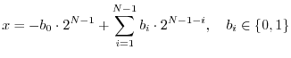
The basic idea of floating point encoding of a binary number is to normalize the number by shifting the bits either left or right until the shifted result lies between 1/2 and 1. (A left-shift by one place in a binary word corresponds to multiplying by 2, while a right-shift one place corresponds to dividing by 2.) The number of bit-positions shifted to normalize the number can be recorded as a signed integer. The negative of this integer (i.e., the shift required to recover the original number) is defined as the exponent of the floating-point encoding. The normalized number between 1/2 and 1 is called the significand, so called because it holds all the ``significant bits'' of the number.
Floating point notation is exactly analogous to ``scientific notation'' for
decimal numbers, e.g.,
![]() ; the number of significant
digits, 5 in this example, is determined by counting digits in the
``significand''
; the number of significant
digits, 5 in this example, is determined by counting digits in the
``significand'' ![]() , while the ``order of magnitude'' is determined by
the power of 10 (-9 in this case). In floating-point numbers, the
significand is stored in fractional two's-complement binary format, and the
exponent is stored as a binary integer.
, while the ``order of magnitude'' is determined by
the power of 10 (-9 in this case). In floating-point numbers, the
significand is stored in fractional two's-complement binary format, and the
exponent is stored as a binary integer.
Since the significand lies in the interval ![]() ,G.6its most significant bit is always a 1, so it is not actually stored in the
computer word, giving one more significant bit of precision.
,G.6its most significant bit is always a 1, so it is not actually stored in the
computer word, giving one more significant bit of precision.
Let's now restate the above a little more precisely. Let ![]() denote a
number to be encoded in floating-point, and let
denote a
number to be encoded in floating-point, and let
![]() denote the normalized value obtained by shifting
denote the normalized value obtained by shifting ![]() either
either ![]() bits to the
right (if
bits to the
right (if ![]() ), or
), or
![]() bits to the left (if
bits to the left (if ![]() ). Then we
have
). Then we
have
![]() , and
, and
![]() . The significand
. The significand
![]() of the floating-point representation for
of the floating-point representation for ![]() is defined as the binary
encoding of
is defined as the binary
encoding of ![]() .G.7 It is
often the case that
.G.7 It is
often the case that ![]() requires more bits than are available for exact
encoding. Therefore, the significand is typically rounded (or
truncated) to the value closest to
requires more bits than are available for exact
encoding. Therefore, the significand is typically rounded (or
truncated) to the value closest to ![]() . Given
. Given ![]() bits for the
significand, the encoding of
bits for the
significand, the encoding of ![]() can be computed by multiplying it by
can be computed by multiplying it by
![]() (left-shifting it
(left-shifting it ![]() bits), rounding to the nearest
integer (or truncating toward minus infinity--as implemented by
the floor() function), and encoding the
bits), rounding to the nearest
integer (or truncating toward minus infinity--as implemented by
the floor() function), and encoding the ![]() -bit result as a binary
(signed) integer.
-bit result as a binary
(signed) integer.
As a final practical note, exponents in floating-point formats may have a
bias. That is, instead of storing ![]() as a binary integer, you may
find a binary encoding of
as a binary integer, you may
find a binary encoding of ![]() where
where ![]() is the bias.G.8
is the bias.G.8
These days, floating-point formats generally follow the IEEE standards set
out for them. A single-precision floating point word is ![]() bits (four
bytes) long, consisting of
bits (four
bytes) long, consisting of ![]() sign bit,
sign bit, ![]() exponent bits, and
exponent bits, and ![]() significand bits, normally laid out as
significand bits, normally laid out as
A double-precision floating point word is ![]() bits (eight bytes) long,
consisting of
bits (eight bytes) long,
consisting of ![]() sign bit,
sign bit, ![]() exponent bits, and
exponent bits, and ![]() significand bits.
In the Intel Pentium processor, there is also an extended precision
format, used for intermediate results, which is
significand bits.
In the Intel Pentium processor, there is also an extended precision
format, used for intermediate results, which is ![]() bits (ten bytes)
containing
bits (ten bytes)
containing ![]() sign bit,
sign bit, ![]() exponent bits, and
exponent bits, and ![]() significand bits. In
Intel processors, the exponent bias is
significand bits. In
Intel processors, the exponent bias is ![]() for single-precision
floating-point,
for single-precision
floating-point, ![]() for double-precision, and
for double-precision, and ![]() for
extended-precision. The single and double precision formats have a
``hidden'' significand bit, while the extended precision format does not.
Thus, the most significant significand bit is always set in extended
precision.
for
extended-precision. The single and double precision formats have a
``hidden'' significand bit, while the extended precision format does not.
Thus, the most significant significand bit is always set in extended
precision.
The MPEG-4 audio compression standard (which supports compression using music synthesis algorithms) specifies that the numerical calculations in any MPEG-4 audio decoder should be at least as accurate as 32-bit single-precision floating point.
Logarithmic Fixed-Point Numbers
In some situations it makes sense to use logarithmic fixed-point. This number format can be regarded as a floating-point format consisting of an exponent and no explicit significand. However, the exponent is not interpreted as an integer as it is in floating point. Instead, it has a fractional part which is a true mantissa. (The integer part is then the ``characteristic'' of the logarithm.) In other words, a logarithmic fixed-point number is a binary encoding of the log-base-2 of the signal-sample magnitude. The sign bit is of course separate.
An example 16-bit logarithmic fixed-point number format suitable for digital audio consists of one sign bit, a 5-bit characteristic, and a 10-bit mantissa:
A nice property of logarithmic fixed-point numbers is that multiplies simply become additions and divisions become subtractions. The hard elementary operation are now addition and subtraction, and these are normally done using table lookups to keep them simple.
One ``catch'' when working with logarithmic fixed-point numbers is that you can't let ``dc'' build up. A wandering dc component will cause the quantization to be coarse even for low-level ``ac'' signals. It's a good idea to make sure dc is always filtered out in logarithmic fixed-point.
Mu-Law Coding
Digital telephone CODECsG.9 have historically used (for land-line switching
networks) a simple 8-bit format called ![]() -law (or simply
``mu-law'') that compresses large amplitudes in a manner loosely
corresponding to human loudness perception.
-law (or simply
``mu-law'') that compresses large amplitudes in a manner loosely
corresponding to human loudness perception.
Given an input sample ![]() represented in some internal format, such as a
short, it is converted to 8-bit mu-law format by the formula
[58]
represented in some internal format, such as a
short, it is converted to 8-bit mu-law format by the formula
[58]
As we all know from talking on the telephone, mu-law sounds really quite good for voice, at least as far as intelligibility is concerned. However, because the telephone bandwidth is only around 3 kHz (nominally 200-3200 Hz), there is very little ``bass'' and no ``highs'' in the spectrum above 4 kHz. This works out fine for intelligibility of voice because the first three formants (envelope peaks) in typical speech spectra occur in this range, and also because the difference in spectral shape (particularly at high frequencies) between consonants such as ``sss'', ``shshsh'', ``fff'', ``ththth'', etc., are sufficiently preserved in this range. As a result of the narrow bandwidth provided for speech, it is sampled at only 8 kHz in standard CODEC chips.
For ``wideband audio'', we like to see sampling rates at least as high as 44.1 kHz, and the latest systems are moving to 96 kHz (mainly because oversampling simplifies signal processing requirements in various areas, not because we can actually hear anything above 20 kHz). In addition, we like the low end to extend at least down to 20 Hz or so. (The lowest note on a normally tuned bass guitar is E1 = 41.2 Hz. The lowest note on a grand piano is A0 = 27.5 Hz.)
Round-Off Error Variance
This appendix shows how to derive that the noise power of amplitude
quantization error is ![]() , where
, where ![]() is the quantization step
size. This is an example of a topic in statistical signal
processing, which is beyond the scope of this book. (Some good
textbooks in this area include
[27,51,34,33,65,32].)
However, since the main result is so useful in practice, it is derived
below anyway, with needed definitions given along the way. The
interested reader is encouraged to explore one or more of the
above-cited references in statistical signal processing.G.10
is the quantization step
size. This is an example of a topic in statistical signal
processing, which is beyond the scope of this book. (Some good
textbooks in this area include
[27,51,34,33,65,32].)
However, since the main result is so useful in practice, it is derived
below anyway, with needed definitions given along the way. The
interested reader is encouraged to explore one or more of the
above-cited references in statistical signal processing.G.10
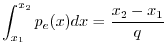
Each round-off error in quantization noise ![]() is modeled as a
uniform random variable between
is modeled as a
uniform random variable between ![]() and
and ![]() . It therefore
has the following probability density function (pdf) [51]:G.11
. It therefore
has the following probability density function (pdf) [51]:G.11
![$\displaystyle p_e(x) = \left\{\begin{array}{ll}
\frac{1}{q}, & \left\vert x\ri...
...2} \\ [5pt]
0, & \left\vert x\right\vert>\frac{q}{2} \\
\end{array} \right.
$](http://www.dsprelated.com/josimages_new/mdft/img2027.png)
The mean of a random variable is defined as
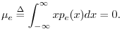
The mean of a signal ![]() is the same thing as the
expected value of
is the same thing as the
expected value of ![]() , which we write as
, which we write as
![]() .
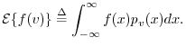
In general, the expected value of any function
.
In general, the expected value of any function ![]() of a
random variable
of a
random variable ![]() is given by
is given by
Since the quantization-noise signal ![]() is modeled as a series of
independent, identically distributed (iid) random variables, we can
estimate the mean by averaging the signal over time.
Such an estimate is called a sample mean.
is modeled as a series of
independent, identically distributed (iid) random variables, we can
estimate the mean by averaging the signal over time.
Such an estimate is called a sample mean.
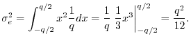
Probability distributions are often characterized by their
moments.
The ![]() th moment of the pdf
th moment of the pdf ![]() is defined as
is defined as
The
variance
of a random variable ![]() is defined as
the
second central moment of the pdf:
is defined as
the
second central moment of the pdf:
![$\displaystyle \sigma_e^2 \isdef {\cal E}\{[e(n)-\mu_e]^2\}
= \int_{-\infty}^{\infty} (x-\mu_e)^2 p_e(x) dx
$](http://www.dsprelated.com/josimages_new/mdft/img2042.png)
Next Section:
Matrices
Previous Section:
Logarithms and Decibels


