


Logarithms and Decibels
This appendix provides an introduction to logarithms (real and complex) and decibels, a quantitative measure of sound intensity. Several specific dB scales are defined, and dynamic range considerations in audio are considered.
Logarithms
A logarithm
![]() is fundamentally an exponent
is fundamentally an exponent
![]() applied to a specific
base
applied to a specific
base
![]() to yield the argument
to yield the argument ![]() .
That is,
.
That is, ![]() . The term ``logarithm'' can be abbreviated as
``log''. The base
. The term ``logarithm'' can be abbreviated as
``log''. The base ![]() is chosen to be a positive real number, and we
normally only take logs of positive real numbers
is chosen to be a positive real number, and we
normally only take logs of positive real numbers ![]() (although it is
ok to say that the log of 0 is
(although it is
ok to say that the log of 0 is ![]() ). The inverse of a
logarithm is called an antilogarithm or antilog; thus,
). The inverse of a
logarithm is called an antilogarithm or antilog; thus,
![]() is the antilog of
is the antilog of ![]() in the base
in the base ![]() .
.
For any positive number ![]() , we have
, we have
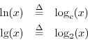
When the base is not specified, it is normally assumed to be ![]() ,
i.e.,
,
i.e.,
![]() . This is the common
logarithm.
. This is the common
logarithm.
Base 2 and base ![]() logarithms have their own special notation:
logarithms have their own special notation:
(The use of ![]() for base
for base ![]() logarithms is common in
computer science. In mathematics, it may denote a base
logarithms is common in
computer science. In mathematics, it may denote a base ![]() logarithm.) By far the most common bases are
logarithm.) By far the most common bases are ![]() ,
, ![]() , and
, and ![]() .
Logs base
.
Logs base ![]() are called natural logarithms. They are
``natural'' in the sense that
are called natural logarithms. They are
``natural'' in the sense that

In general, a logarithm ![]() has an integer part and a fractional part.
The integer part is called the
characteristic of the logarithm,
and the fractional part is called the mantissa. These terms
were suggested by Henry Briggs in 1624. ``Mantissa'' is a Latin word
meaning ``addition'' or ``make weight''--something added to make up
the weight [28].
has an integer part and a fractional part.
The integer part is called the
characteristic of the logarithm,
and the fractional part is called the mantissa. These terms
were suggested by Henry Briggs in 1624. ``Mantissa'' is a Latin word
meaning ``addition'' or ``make weight''--something added to make up
the weight [28].
The following Matlab code illustrates splitting a natural logarithm into its characteristic and mantissa:
>> x = log(3)
   x = 1.0986
>> characteristic = floor(x)
   characteristic = 1
>> mantissa = x - characteristic
   mantissa = 0.0986

>> % Now do a negative-log example
>> x = log(0.05)
   x = -2.9957
>> characteristic = floor(x)
   characteristic = -3
>> mantissa = x - characteristic
   mantissa = 0.0043
Logarithms were used in the days before computers to perform
multiplication of large numbers. Since
![]() , one can look up the logs of
, one can look up the logs of ![]() and
and ![]() in tables of
logarithms, add them together (which is easier than multiplying), and
look up the antilog of the result to obtain the product
in tables of
logarithms, add them together (which is easier than multiplying), and
look up the antilog of the result to obtain the product ![]() . Log
tables are still used in modern computing environments to replace
expensive multiplies with less-expensive table lookups and additions.
This is a classic trade-off between memory (for the log tables) and
computation. Nowadays, large numbers are multiplied using FFT
fast-convolution techniques.
. Log
tables are still used in modern computing environments to replace
expensive multiplies with less-expensive table lookups and additions.
This is a classic trade-off between memory (for the log tables) and
computation. Nowadays, large numbers are multiplied using FFT
fast-convolution techniques.
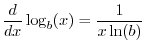
Changing the Base
By definition,
![]() . Taking the log base
. Taking the log base ![]() of both sides
gives
of both sides
gives
Logarithms of Negative and Imaginary Numbers
By Euler's identity,
![]() , so that
, so that
Similarly,
![]() , so that
, so that
Finally, from the polar representation
![]() for
complex numbers,
for
complex numbers,
Decibels
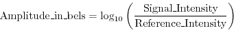
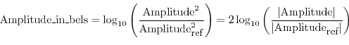
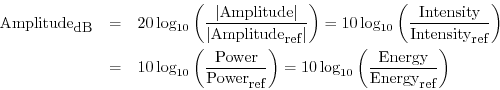
A decibel (abbreviated dB) is defined as one tenth of a bel. The belF.1 is an amplitude unit defined for sound as the log (base 10) of the intensity relative to some reference intensity,F.2 i.e.,
A just-noticeable difference (JND) in amplitude level is on the order of a quarter dB. In the early days of telephony, one dB was considered a reasonable ``smallest step'' in amplitude, but in reality, a series of half-dB amplitude steps does not sound very smooth, while quarter-dB steps do sound pretty smooth. A typical professional audio filter-design specification for ``ripple in the passband'' is 0.1 dB.
Properties of DB Scales
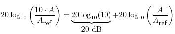
In every kind of dB, a factor of 10 in amplitude increase corresponds to a 20 dB boost (increase by 20 dB):
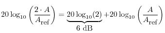
Similarly, a factor of 2 in amplitude gain corresponds to a 6 dB boost:
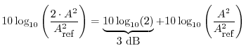
A doubling of power corresponds to a 3 dB boost:
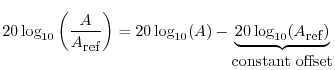
Finally, note that the choice of reference merely determines a vertical offset in the dB scale:
Specific DB Scales
Since we so often rescale our signals to suit various needs (avoiding
overflow, reducing quantization noise, making a nicer plot, etc.),
there seems to be little point in worrying about what the dB reference
is--we simply choose it implicitly when we rescale to obtain signal
values in the range we want to see. In particular, dB relative
to full scale (
![]() ), abbreviated
dBFS, is perhaps the most commonly used case in the digital
audio world. Thus, 0 dBFS means maximum amplitude, and typical
amplitude levels are negative in dBFS. In addition, there are a few
specific dB scales that are worth knowing about.
), abbreviated
dBFS, is perhaps the most commonly used case in the digital
audio world. Thus, 0 dBFS means maximum amplitude, and typical
amplitude levels are negative in dBFS. In addition, there are a few
specific dB scales that are worth knowing about.
DBm Scale
One common dB scale in audio recording is the dBm scale in which the reference power is taken to be a milliwatt (1 mW) dissipated by a 600 Ohm resistor. (See §F.3 for a primer on resistors, voltage, current, and power.)
DBV Scale
Another dB scale is the dBV scale which sets 0 dBV to 1 volt. Thus, a 100-volt signal is
 40 dBV
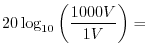 60 dBV
DB SPL
Sound Pressure Level (SPL) is defined using a reference which is approximately the intensity of 1000 Hz sinusoid that is just barely audible (zero ``phons''). In pressure units:F.3
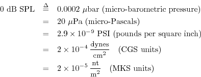
In intensity units:
Since sound is created by a time-varying pressure, we compute sound levels in dB-SPL by using the average intensity (averaged over at least one period of the lowest frequency contained in the sound).
Table F.1 gives a list of common sound levels and their dB
equivalents [54]:
|
In my experience, the ``threshold of pain'' is most often defined as 120 dB.
The relationship between sound amplitude and actual loudness is complex [76]. Loudness is a perceptual dimension while sound amplitude is physical. Since loudness sensitivity is closer to logarithmic than linear in amplitude (especially at moderate to high loudnesses), we typically use decibels to represent sound amplitude, especially in spectral displays.
The sone amplitude scale is defined in terms of actual loudness perception experiments [76]. At 1kHz and above, loudness perception is approximately logarithmic above 50 dB SPL or so. Below that, it tends toward being more linear.
The phon amplitude scale is simply the dB scale at 1kHz [76, p. 111]. At other frequencies, the amplitude in phons is defined by following the equal-loudness curve over to 1 kHz and reading off the level there in dB SPL. In other words, all pure tones have the same loudness at the same phon level, and 1 kHz is used to set the reference in dB SPL. Just remember that one phon is one dB-SPL at 1 kHz. Looking at the Fletcher-Munson equal-loudness curves [76, p. 124], loudness in phons can be read off along the vertical line at 1 kHz.
Classically, the intensity level of a sound wave is its dB SPL
level, measuring the peak time-domain pressure-wave amplitude relative to
![]() watts per centimeter squared (i.e., there is no consideration of
the frequency domain here at all).
watts per centimeter squared (i.e., there is no consideration of
the frequency domain here at all).
Another classical term still encountered is the sensation level of pure tones: The sensation level is the number of dB SPL above the hearing threshold at that frequency [76, p. 110].
For further information on ``doing it right,'' see, for example,
http://www.measure.demon.co.uk/Acoustics_Software/loudness.html.
DBA (A-Weighted DB)
The so-called A-weighted dB scale (abbreviated dBA) is based on the Fletcher-Munson equal-loudness curve for an SPL of 40 phons.F.4 Thus, a dBA weighting assumes a fairly quiet pure tone. Despite this assumption, the dBA weighting is often used as an approximate equal loudness adjustment for measured spectra.
An analog filter transfer function that can be used to implement an approximate A-weighting is given byF.5

The ITU-R 468 noise weightingF.6is said to perform better for measuring noise in audio systems.
DB for Display
In practical signal processing, it is common to choose the maximum signal magnitude as the reference amplitude. That is, we normalize the signal so that the maximum amplitude is defined as 1, or 0 dB. This convention is also used by ``sound level meters'' in audio recording. When displaying magnitude spectra, the highest spectral peak is often normalized to 0 dB. We can then easily read off lower peaks as so many dB below the highest peak.
Figure F.1b shows a plot of the Fast Fourier Transform (FFT) of
ten periods of a ``Kaiser-windowed'' sinusoid at ![]() Hz. (FFT
windows are introduced in §8.1.4.
The window is used to
taper a finite-duration section of the signal.) Note that the peak dB
magnitude has been normalized to zero, and that the plot has been
clipped at -100 dB.
Hz. (FFT
windows are introduced in §8.1.4.
The window is used to
taper a finite-duration section of the signal.) Note that the peak dB
magnitude has been normalized to zero, and that the plot has been
clipped at -100 dB.
![\includegraphics[width=\twidth]{eps/freqdpy}](http://www.dsprelated.com/josimages_new/mdft/img1954.png)
Below is the Matlab code for producing Fig.F.1. Note that it contains several elements (windows, zero padding, spectral interpolation) that we will not cover until later. They are included here as ``forward references'' in order to keep the example realistic and practical, and to give you an idea of ``how far we have to go'' before we know how to do practical spectrum analysis. Otherwise, the example just illustrates plotting spectra on an arbitrary dB scale between convenient limits.
% Practical display of the fft of a synthesized sinusoid

fs = 44100;             % Sampling rate
f = 440;                % Sinusoidal frequency = A-440
nper = 10;              % Number of periods to synthesize
dur = nper/f;           % Duration in seconds
T = 1/fs;               % Sampling period
t = 0:T:dur;            % Discrete-time axis in seconds
L = length(t)           % Number of samples to synthesize
ZP = 5;                 % Zero padding factor
N = 2^(nextpow2(L*ZP))  % FFT size (power of 2)

x = cos(2*pi*f*t);      % A sinusoid at A-440 ("row vector")
w = kaiser(L,8);        % An "FFT window"
xw = x .* w';           % Need to transpose w to get a row
sound(xw,fs);           % Might as well listen to it
xzp = [xw,zeros(1,N-L)];% Zero-padded FFT input buffer
X = fft(xzp);           % Interpolated spectrum of xw

Xmag = abs(X);          % Spectral magnitude
Xdb = 20*log10(Xmag);   % Spectral magnitude in dB

XdbMax = max(Xdb);      % Peak dB magnitude
Xdbn = Xdb - XdbMax;    % Normalize to 0dB peak

dBmin = -100;           % Don't show anything lower than this
Xdbp = max(Xdbn,dBmin); % Normalized, clipped, dB mag spec
fmaxp = 2*f;            % Upper frequency limit of plot, Hz
kmaxp = fmaxp*N/fs;     % Upper frequency limit of plot, bins
fp = fs*[0:kmaxp]/N;    % Frequency axis in Hz

% Ok, plot it already!

subplot(2,1,1);
plot(1000*t,xw);
xlabel('Time (ms)');
ylabel('Amplitude');
title(sprintf(['a) %d Periods of a %3.0f Hz Sinusoid, ',
               'Kaiser Windowed'],nper,f)R);

subplot(2,1,2);
plot(fp,Xdbp(1:kmaxp+1)); grid;
% Plot a dashed line where the peak should be:
  hold on; plot([440 440],[dBmin,0],'--'); hold off;
xlabel('Frequency (Hz)');
ylabel('Magnitude (dB)');
title(sprintf(['b) Interpolated FFT of %d Periods of ',...
        '%3.0f Hz Sinusoid'],nper,f));
The following more compact Matlab produces essentially the same plot, but without the nice physical units on the horizontal axes:
x = cos([0:2*pi/20:10*2*pi]); % 10 periods, 20 samples/cycle
L = length(x);
xw = x' .* kaiser(L,8);
N = 2^nextpow2(L*5);
X = fft([xw',zeros(1,N-L)]);

subplot(2,1,1); plot(xw);
xlabel('Time (samples)'); ylabel('Amplitude');
title('a) 10 Periods of a Kaiser-Windowed Sinusoid');

subplot(2,1,2); kmaxp = 2*10*5; Xl = 20*log10(abs(X(1:kmaxp+1)));
plot([10*5+1,10*5+1],[-100,0],[0:kmaxp],max(Xl-max(Xl),-100)); grid;
xlabel('Frequency (Bins)'); ylabel('Magnitude (dB)');
title('b) Interpolated FFT of 10 Periods of Sinusoid');
Dynamic Range
The dynamic range of a signal processing system can be defined as the maximum dB level sustainable without overflow (or other distortion) minus the dB level of the ``noise floor''.
Similarly, the dynamic range of a signal can be defined as its maximum decibel level minus its average ``noise level'' in dB. For digital signals, the limiting noise is ideally quantization noise.
Quantization noise is generally modeled as a uniform random variable
between plus and minus half the least significant bit (since rounding to
the nearest representable sample value is normally used). If ![]() denotes
the quantization interval, then the maximum quantization-error magnitude is
denotes
the quantization interval, then the maximum quantization-error magnitude is
![]() , and its variance (``noise power'') is
, and its variance (``noise power'') is
![]() (see
§G.3 for a derivation of this value).
(see
§G.3 for a derivation of this value).
The rms level of the quantization noise is therefore
![]() , or about 60% of the maximum error.
, or about 60% of the maximum error.
The number system (see Appendix G and number of bits chosen to represent signal samples determines their available dynamic range. Signal processing operations such as digital filtering may use the same number system as the input signal, or they may use extra bits in the computations, yielding an increased ``internal dynamic range''.
Since the threshold of hearing is near 0 dB SPL, and since the ``threshold of pain'' is often defined as 120 dB SPL, we may say that the dynamic range of human hearing is approximately 120 dB.
The dynamic range of magnetic tape is approximately 55 dB. To increase the dynamic range available for analog recording on magnetic tape, companding is often used. ``Dolby A'' adds approximately 10 dB to the dynamic range that will fit on magnetic tape (by compressing the signal dynamic range by 10 dB), while DBX adds 30 dB (at the cost of more ``transient distortion'').F.7 In general, any dynamic range can be mapped to any other dynamic range, subject only to noise limitations.
Voltage, Current, and Resistance
The state of an ideal resistor is completely specified by the voltage
across it (call it ![]() volts) and the current passing through
it (
volts) and the current passing through
it (![]() amperes, or simply ``amps''). The ratio of voltage to
current gives the value of the resistor (
amperes, or simply ``amps''). The ratio of voltage to
current gives the value of the resistor (![]() resistance in
Ohms). The fundamental relation between voltage and current in a
resistor is called
Ohm's Law:
resistance in
Ohms). The fundamental relation between voltage and current in a
resistor is called
Ohm's Law:
The electrical power in watts dissipated by a resistor R is given by

Exercises
- Show that
where
 denotes the logarithm to the base
  of
of  .
.
- Work out the definition of logarithms using a complex base .
- Try synthesizing a sawtooth waveform which increases by 1/2
dB a few times per second, and again using 1/4 dB increments. See if
you agree that quarter-dB increments are ``smooth'' enough for you.
Next Section:
Number Systems for Digital Audio
Previous Section:
Taylor Series Expansions


