


Digitizing Elementary Reflectances by Bilinear Transform
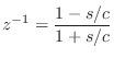
Going to discrete time via the bilinear transform means making the substitution
 |
(F.11) |
where
Solving for ![]() gives us the inverse bilinear transform:
gives us the inverse bilinear transform:
In this case, we see that setting ![]() further simplifies our
universal reflectances in the digital domain:
further simplifies our
universal reflectances in the digital domain:
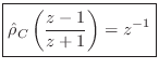
- For the ``wave digital capacitor'' (or spring), Eq.
 (F.8) becomes
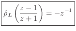
- For the ``wave digital inductor'' (or mass), Eq.(F.9) becomes
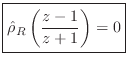
- And for the ``wave digital resistor'' (or dashpot), Eq.(F.10) becomes
as before in the continuous-time case.
Note that this choice of ![]() is also the only one that eliminates
delay-free paths in the fundamental elements. This allows them to
be used as building blocks for explicit finite difference
schemes.
is also the only one that eliminates
delay-free paths in the fundamental elements. This allows them to
be used as building blocks for explicit finite difference
schemes.
We may still obtain the above results using the more typical value
![]() (instead of
(instead of ![]() ) in the bilinear transform. From
Eq.
) in the bilinear transform. From
Eq.![]() (F.12), it is clear that changing
(F.12), it is clear that changing ![]() amounts to a linear
frequency scaling of
amounts to a linear
frequency scaling of ![]() . Such a scaling may be compensated
by choosing the waveguide (port) impedances to be
. Such a scaling may be compensated
by choosing the waveguide (port) impedances to be
![]() (instead of
(instead of ![]() ) for the inductor, and
) for the inductor, and
![]() (instead of
(instead of
![]() ) for the capacitor.
) for the capacitor.
Next Section:
Compatible Port Connections
Previous Section:
Choosing Impedance to Simplify Element Reflectance


