


Wave Digital Dashpot
Starting with a dashpot with coefficient ![]() , we have
, we have
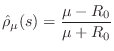
In the context of waveguide theory, a zero reflectance corresponds to a matched impedance, i.e., the terminating transmission-line impedance equals the characteristic impedance of the line.
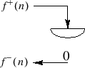
The difference equation for the wave digital dashpot is simply
![]() . While this may appear overly degenerate at first,
remember that the interface to the element is a port at impedance
. While this may appear overly degenerate at first,
remember that the interface to the element is a port at impedance
![]() . Thus, in this particular case only, the infinitesimal
waveguide interface is the element itself.
. Thus, in this particular case only, the infinitesimal
waveguide interface is the element itself.
Next Section:
Limiting Cases
Previous Section:
Wave Digital Spring


