In (9.19) of the previous section, we derived that the FBS
reconstruction sum gives
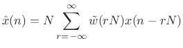 |
(10.20) |
where
. From this we see that if

(where

is
the window length and

is the
DFT size), as is normally the case,
then

for
. This is the
Fourier dual
of the ``strong
COLA constraint'' for OLA (see
§
8.3.2). When it holds, we have
 |
(10.21) |
This is simply a gain term, and so we are able to recover the original
signal exactly. (
Zero-phase windows are appropriate here.)
If the window length is larger than the number of analysis frequencies
( ), we can still obtain perfect reconstruction provided
![$\displaystyle w(rN) = 0, \hspace{1cm} \vert r\vert=1,2,\dots \qquad\hbox{[$w$\ is Nyquist($N$)]}$](http://www.dsprelated.com/josimages_new/sasp2/img1626.png) |
(10.22) |
When this holds, we say the window is
. (This is the dual of
the weak
COLA constraint introduced in §
8.3.1.)
Portnoff windows, discussed
in §
9.7, make use of this result; they are
longer than the DFT size and therefore must be used in
time-aliased form [
62]. An advantage of
Portnoff windows is that they give reduced overlap among the channel
filter pass-bands. In the limit, a Portnoff window can approach a
sinc
function having its zero-crossings at all nonzero multiples of
samples, thereby yielding an ideal channel filter with
bandwidth

. Figure
9.16 compares example Hamming and Portnoff
windows.
Figure 3.35:
![\includegraphics[width=\twidth]{eps/colawin}](http://www.dsprelated.com/josimages_new/sasp2/img1628.png) |
Next Section: Duality of COLA and Nyquist ConditionsPrevious Section: FBS Window Constraints for R=1


