


Poisson Summation Formula
Consider the summation of N complex sinusoids having frequencies uniformly spaced around the unit circle [264]:
![\begin{eqnarray*}
x(n) &\mathrel{\stackrel{\Delta}{=}}& \frac{1}{N} \sum_{k=0}^{N-1}e^{j\omega_kn} =
\left\{
\begin{array}{ll}
1 & n=0 \quad (\hbox{\sc mod}\ N) \\
0 & \mbox{elsewhere} \\
\end{array} \right. \\ [5pt]
&=& \hbox{\sc IDFT}_n(1 \cdots 1)
\end{eqnarray*}](http://www.dsprelated.com/josimages_new/sasp2/img1454.png)
where
 .
.
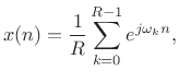
![\begin{psfrags}
% latex2html id marker 22700\psfrag{d(n)}{\normalsize $\displaystyle\normalsize \sum_l\delta(n-lN)$\ }\psfrag{\makebox[0pt][l]{2}N}{\normalsize $-2N$}\psfrag{\makebox[0pt][l]{N}}{\normalsize $-N$}\psfrag{0}{\normalsize $0$}\psfrag{N}{\normalsize $N$}\psfrag{n}{\normalsize $n$}\psfrag{2N}{\normalsize $2N$}\psfrag{1}{\normalsize $1$}\begin{figure}[htbp]
\includegraphics[width=3.5in]{eps/delta}
\caption{Discrete-time impulse train created
by a sum of sampled complex sinusoids.}
\end{figure}
\end{psfrags}](http://www.dsprelated.com/josimages_new/sasp2/img1456.png)
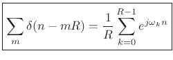
Setting ![]() (the FFT hop size) gives
(the FFT hop size) gives
 |
(9.26) |
where
 (harmonics of the frame rate).
Let us now consider these equivalent signals as inputs to an LTI
system, with an impulse response given by ![]() , and frequency response
equal to
, and frequency response
equal to ![]() .
.
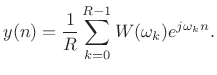
![\begin{psfrags}
% latex2html id marker 22729\psfrag{w(n)}{\normalsize $w(n)$\ }\psfrag{W(w)}{\normalsize $W(\omega)$\ }\psfrag{timesum}{\normalsize $\displaystyle\sum_l\delta(n-lR)$\ }\psfrag{freqsum}{\normalsize $\frac{1}{R}\displaystyle\sum_k e^{j\omega_kn}$\ }\psfrag{t}{\normalsize $\displaystyle\sum_l w(n-lR)$\ }\psfrag{f}{\normalsize $\frac{1}{R}\displaystyle\sum_k W(\omega_k)e^{j\omega_kn}$\ }\psfrag{time}{\normalsize Time}\psfrag{freq}{\normalsize Frequency}\begin{figure}[htbp]
\includegraphics[width=4in]{eps/poisson}
\caption{Linear systems theory proof of the Poisson summation formula.}
\end{figure}
\end{psfrags}](http://www.dsprelated.com/josimages_new/sasp2/img1460.png)
Looking across the top of Fig.8.16, for the case of input signal
![]() we have
we have
 |
(9.27) |
Looking across the bottom of the figure, for the case of input signal
 |
(9.28) |
we have the output signal
 |
(9.29) |
This second form follows from the fact that complex sinusoids
Since the inputs were equal, the corresponding outputs must be equal too. This derives the Poisson Summation Formula (PSF):
![$\displaystyle \zbox {\underbrace{\sum_m w(n-mR)}_{\hbox{\sc Alias}_R(w)} = \underbrace{\frac{1}{R}\sum_{k=0}^{R-1} W(\omega_k)e^{j\omega_k n}}_{\hbox{\sc DFT}_R^{-1} \left[\hbox{\sc Sample}_{\frac{2\pi}{R}}(W)\right]}} \quad \omega_k \isdef \frac{2\pi k}{R} \protect$](http://www.dsprelated.com/josimages_new/sasp2/img1466.png)
Note that the PSF is the Fourier dual of the sampling theorem [270], [264, Appendix G].
The continuous-time PSF is derived in §B.15.
Next Section:
Frequency-Domain COLA Constraints
Previous Section:
Summary of Overlap-Add FFT Processing


