


Poisson Summation Formula
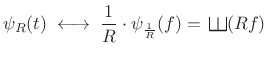
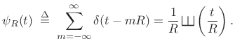
As shown in §B.14 above, the Fourier transform of an impulse train is an impulse train with inversely proportional spacing:
 |
(B.56) |
where
 |
(B.57) |
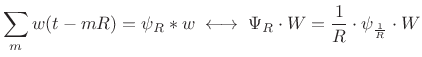
Using this Fourier theorem, we can derive the continuous-time PSF using the convolution theorem for Fourier transforms:B.1
 |
(B.58) |
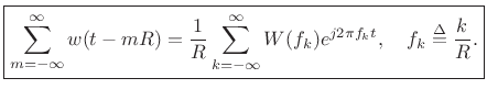
Using linearity and the shift theorem for inverse Fourier transforms, the above relation yields
![\begin{eqnarray*}
\sum_m w(t-mR)
&=& \frac{1}{R} \hbox{\sc IFT}_t
\left[W(f)\sum_k\delta\left(f-k\frac{1}{R}\right) \right]
\quad\left(\mbox{define $f_k\isdef \frac{k}{R}$}\right)
\\ [5pt]
&=& \frac{1}{R} \hbox{\sc IFT}_t
\left[\sum_k W(f_k)\cdot\delta\left(f-f_k\right) \right]\\ [5pt]
&=& \frac{1}{R}
\sum_k W(f_k)\cdot\hbox{\sc IFT}_t \left[\delta\left(f-f_k\right) \right]\\ [5pt]
&=& \frac{1}{R} \sum_k W(f_k)e^{j 2\pi f_k t}.
\end{eqnarray*}](http://www.dsprelated.com/josimages_new/sasp2/img2530.png)
We have therefore shown
Compare this result to Eq.
Next Section:
Sampling Theory
Previous Section:
Impulse Trains


