


Sample-Mean Variance
The simplest case to study first is the sample mean:
 |
(C.29) |
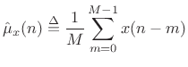
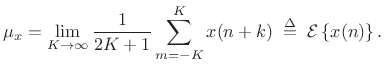
Here we have defined the sample mean at time
| (C.30) |
or
 |
(C.31) |
Now assume
Var![$\displaystyle \left\{x(n)\right\} \isdefs {\cal E}\left\{[x(n)-\mu_x]^2\right\} \eqsp {\cal E}\left\{x^2(n)\right\} \eqsp \sigma_x^2$](http://www.dsprelated.com/josimages_new/sasp2/img2697.png) |
(C.32) |
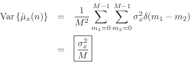
Then the variance of our sample-mean estimator
![]() can be calculated as follows:
can be calculated as follows:
![\begin{eqnarray*}
\mbox{Var}\left\{\hat{\mu}_x(n)\right\} &\isdef & {\cal E}\left\{\left[\hat{\mu}_x(n)-\mu_x \right]^2\right\}
\eqsp {\cal E}\left\{\hat{\mu}_x^2(n)\right\}\\
&=&{\cal E}\left\{\frac{1}{M}\sum_{m_1=0}^{M-1} x(n-m_1)\,
\frac{1}{M}\sum_{m_2=0}^{M-1} x(n-m_2)\right\}\\
&=&\frac{1}{M^2}\sum_{m_1=0}^{M-1}\sum_{m_2=0}^{M-1}
{\cal E}\left\{x(n-m_1) x(n-m_2)\right\}\\
&=&\frac{1}{M^2}\sum_{m_1=0}^{M-1}\sum_{m_2=0}^{M-1}
r_x(\vert m_1-m_2\vert)
\end{eqnarray*}](http://www.dsprelated.com/josimages_new/sasp2/img2699.png)
where we used the fact that the time-averaging operator
![]() is
linear, and
is
linear, and ![]() denotes the unbiased autocorrelation of
denotes the unbiased autocorrelation of ![]() .
If
.
If ![]() is white noise, then
is white noise, then
![]() , and we obtain
, and we obtain
We have derived that the variance of the ![]() -sample running average of
a white-noise sequence
-sample running average of
a white-noise sequence ![]() is given by
is given by
![]() , where
, where
![]() denotes the variance of
denotes the variance of ![]() . We found that the
variance is inversely proportional to the number of samples used to
form the estimate. This is how averaging reduces variance in general:
When averaging
. We found that the
variance is inversely proportional to the number of samples used to
form the estimate. This is how averaging reduces variance in general:
When averaging ![]() independent (or merely uncorrelated) random
variables, the variance of the average is proportional to the variance
of each individual random variable divided by
independent (or merely uncorrelated) random
variables, the variance of the average is proportional to the variance
of each individual random variable divided by ![]() .
.
Next Section:
Sample-Variance Variance
Previous Section:
Generalized STFT


