Round Round Get Around: Why Fixed-Point Right-Shifts Are Just Fine

Today’s topic is rounding in embedded systems, or more specifically, why you don’t need to worry about it in many cases.

One of the issues faced in computer arithmetic is that exact arithmetic requires an ever-increasing bit length to avoid overflow. Adding or subtracting two 16-bit integers produces a 17-bit result; multiplying two 16-bit integers produces a 32-bit result. In fixed-point arithmetic we typically multiply and shift right; for example, if we wanted to multiply some number \( x \) by 0.98765, we could approximate by computing (K * x) >> 15 where \( K \approx 0.98765 \times 2^{15} \):

K_exact = 0.98765
K = K_exact * (1 << 15)
K

32363.3152

x = 2016
x*K_exact

1991.1024

(x * 32363) >> 15

1991

Whee, close enough. As I’ve said before:

The only embedded systems that require precision floating-point computations are desktop calculators.

Now, when we performed this calculation, we made two approximations in which we had to throw away information and avoid the need to increase storage sizes.

One was a design-time approximation, where we decided that \( K = 32363 \) was a good enough approximation to \( 0.98765 \times 2^{15} = 32363.3152 \). (I’m not going to get rigorous on this stuff, by the way; if you want rigor, read Knuth’s The Art of Computer Programming, volume 2, covering floating-point arithmetic, where he distinguishes exact operations \( +, -, \times, \div \) from the computer’s floating-point arithmetic operations \( \oplus, \ominus, \otimes, \oslash \), and gets into ulp and \( \delta \) and \( \epsilon \) and things like that.)

The other was a runtime approximation, that the computing environment’s right-shift >> operator was an appropriate way to divide by \( 2^{15} \) and discard the least significant bits; the exact computation does not produce an integer result:

(x * 32363) / 32768.0

1991.0830078125

You look at these numbers and say of course, 32363 is a good approximation to 32363.3152, and 1991 is a good approximation to 1991.0830078125. But that’s because in both cases, truncating (just throwing away the low-order bits or digits) happened to give us the integer values that are closest to the exact numbers we’re trying to approximate. Truncation is only one way to handle approximation by integers. It’s also usually the easiest way, since computer languages such as C or Python use truncation when handling integer division and right-shifting, and the underlying computer architectures have an arithmetic logic unit (ALU) that does the same… which is why the computer languages tend to have identical behavior, so they can both mirror and make efficient use of their underlying hardware.

Actually, we need to be a little careful here. Truncation is tricky, because it’s not the same operation when you deal with printed numbers and their two’s complement representations in a computer, at least not when negative numbers are involved. Numerical truncation to an integer is throwing away the digits to the right of the decimal point, effectively rounding towards zero. Bitwise truncation is throwing away all the bits to the right of the binary point, which with two’s complement representation always rounds downward. If we had the number -3.34375, this could be represented exactly in two’s complement as 11111100.10101000 which truncates to 11111100 = -4.

int('1111110010101000',2) / 256.0 - 256

-3.34375

Anyway, all the numbers turned out nicely in the examples above. But suppose we wanted to multiply by 0.56789:

0.56789 * (1<<15)

18608.61952

Now we have a choice. We could use \( K = 18608 \), which we obtained by truncation. Or we could use \( K = 18609 \), which we obtained by rounding to the nearest integer; this has a smaller error.

As far as the result of our fixed-point multiplication goes:

print "exact: ", 0.56789*x
for K in [18608, 18609]:
    print (K * x) / 32768.0

exact:  1144.86624
1144.828125
1144.88964844

Again, we have a choice; we could use bitwise truncation and round down to 1144. Or we could round to the nearest integer to 1145, which has smaller error.

For design-time calculations, where there’s almost no cost, because we can do them on a PC and we only need to go through them once, it is always better to round to the nearest integer rather than round down. There are, however, rare occasions where rounding towards zero is a better approach, because of other constraints that allow us to reduce but not increase the magnitude of the numbers involved. (Rotation matrix coefficients, for example, in a series of fixed-point iterations, have the potential to make their output larger, risking overflow, if they are rounded to the nearest integer, whereas rounding towards zero guarantees that each iteration does not increase in magnitude.)

Runtime calculations, on the other hand, have a slight increase in cost for rounding compared to bitwise truncation. This is because the operation of fixed-point rounding to the nearest integer is not a common feature, either in microcontroller architectures or computer languages (and not present in C: the behavior of the division and right-shift operators exclude rounding). Achieving round-to-the-nearest-integer behavior isn’t hard though; when right-shifting by \( N \), just add in \( 2^{N-1} \) (which is the fixed-point equivalent of 0.5) first:

print (18608 * x) >> 15
print (18608 * x + 16384) >> 15

1144
1145

This costs an extra operation, which can add up on an embedded system, and some specialized DSP instructions on certain architectures — the SAC.R instruction on Microchip’s dsPIC30F and dsPIC33 cores, for example — do include automatic rounding facilities. (Floating-point rounding modes, on the other hand, do appear to be common in many architectures, primarily because they were written into the IEEE-754 standard and even included in standard libraries in C and C++ and Java.)

If accuracy is very important, rounding-to-nearest-integer at runtime will produce an integer result that has smaller error than bitwise truncation. My contention is that this is not necessary in many applications, and I will explain why in a moment.

Biased vs. unbiased rounding

The technique of adding 0.5 and then rounding down (round(x) = floor(x+0.5)) is fairly common, and in many PC calculations, that’s all that’s needed. For some applications this isn’t enough, because this type of rounding is biased, namely values of exactly \( m + 0.5 \) for integer \( m \) will always round to \( m+1 \), creating a small positive bias in the average error over the set of input operands. One technique for unbiased rounding is when encountering these numbers that are exactly halfway between integers, round to the nearest even integer, namely:

$$ \begin{array}{rcr} \mathrm{round}(-3.5) & \rightarrow & -4\cr \mathrm{round}(-2.5) & \rightarrow & -2\cr \mathrm{round}(-1.5) & \rightarrow & -2\cr \mathrm{round}(-0.5) & \rightarrow & 0\cr \mathrm{round}(+0.5) & \rightarrow & 0\cr \mathrm{round}(+1.5) & \rightarrow & 2\cr \mathrm{round}(+2.5) & \rightarrow & 2\cr \mathrm{round}(+3.5) & \rightarrow & 4\cr \end{array} $$

This ensures there is no net bias, and the average error over extremely large numbers of calculations, with inputs well-distributed, is zero.

That sounds a bit pedantic, especially in the floating-point world, where encountering numbers exactly between two integers seems extremely rare. Knuth points out, however, in TAOCP (section 4.2.2 in the Third Edition) that

No rounding rule can be best for every application. For example, we generally want a special rule when computing our income tax. But for most numerical calculations the best policy appears to be the rounding scheme specified in Algorithm 4.2.1N, which insists that the least significant digit should always be made even (or always odd) when an ambiguous value is rounded. This is not a trivial technicality, of interest only to nit-pickers; it is an important practical consideration, since the ambiguous case arises surprisingly often and a biased rounding rule produces significantly poor results. For example, consider decimal arithmetic and assume that remainders of 5 are always rounded upwards. Then if \( u = 1.0000000 \) and \( v = 0.55555555 \) we have \( u \oplus v = 1.5555556 \); and if we floating-subtract \( v \) from this result we get \( u’ = 1.0000001 \). Adding and subtracting \( v \) from \( u’ \) gives 1.0000002, and the next time we get 1.0000003, etc.; the result keeps growing although we are adding and subtracting the same value.

This phenomenon, called drift, will not occur when we use a stable rounding rule based on the parity of the least significant digit. More precisely:

Theorem D. \( \bigl(\left(\left(u \oplus v\right) \ominus v\right) \oplus v\bigr) \ominus v = (u \oplus v) \ominus v \).

For example, if \( u = 1.2345679 \) and \( v = -0.23456785 \), we find

$$\begin{array}{rclrcl} u\oplus v &=& 1.0000000, & (u\oplus v) \ominus v &=& 1.2345678, \cr \left(\left(u\oplus v\right)\ominus v\right) \oplus v &=& 1.0000000, & \bigl(\left(\left(u\oplus v\right) \ominus v\right) \oplus v\bigr) \ominus v &=& 1.2345678. \cr \end{array}$$ The proof for general \( u \) and \( v \) seems to require a case analysis even more detailed than that in the theorems above; see the references below.

Aside from the rigorous theory, which may turn off some readers, this is the only account I have found of why unbiased rounding is important; it’s not just some statistical thing where if you sum up one trillion numbers you’re off by 0.001%, but rather there are relatively simple situations in which small errors can accumulate.

Rounding in embedded systems

Okay, here we get to the practical stuff.

My assertion is that you don’t need rounding in the vast majority of cases in embedded systems; bitwise truncation is just fine. Why? Because there are other errors which are much larger, and drown out the errors caused by truncation. It’s like dusting the shelves and washing the floors in a house, before you bring a couple of sheep inside along with some hay bales. Or trying to walk silently when someone’s playing Won’t Get Fooled Again loudly on their stereo. I mean, what’s the point?

Let’s look at an example, again multiplication by 0.98765, so we’re comparing

$$\begin{eqnarray} y &=& 0.98765x \cr y_{t} &=& \left\lfloor \frac{32363x}{32768} \right\rfloor \cr y_{r} &=& \left\lfloor \frac{32363x}{32768} + 0.5 \right\rfloor \end{eqnarray}$$

import numpy as np
import matplotlib.pyplot as plt

xmin = -2048
xmax = 2048
x = np.arange(xmin,xmax)
y = x*0.98765
fig=plt.figure()
for k,ofs,subscript in ([1,0,'t'],[2,16384,'r']):
    yq = (x*32363 + ofs) >> 15
    ax=fig.add_subplot(2,1,k)
    ax.plot(x,y-yq)
    ax.set_xlim(xmin,xmax)
    ax.set_xlabel('$x$',fontsize=18)
    ax.set_ylabel('$\\tilde{y} = y-y_%s$' % subscript, fontsize=18)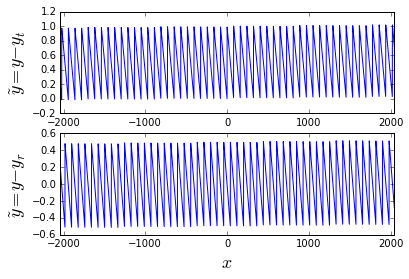

It’s pretty easy to see the results; in the case of truncation the error band is essentially between 0 and 1 count; in the case of rounding, the error band is essentially between -0.5 and 0.5 counts. I say “essentially” because there is a small gain error because we’re multiplying by 32363/32768 instead of exactly 0.98765.

In any case, we have an error with a peak-to-peak value of 1 count. Bitwise truncation puts the error band between 0 and 1 count, with a mean bias of 0.5 counts; simple rounding to the nearest integer brings the mean bias down to essentially \( 1/2^{-Q} = 1/32768 \) counts where \( Q \) is the right-shift count; we need unbiased rounding if we want to have a mean bias of zero.

Now let’s say that we get our input \( x \) from an analog-to-digital converter (ADC). The ADC itself is going to have some offset error, typically in the neighborhood of 1-10 counts depending on the number of bits, and integral and differential nonlinearity of several counts. Let’s say I use a dsPIC33EP256MC506 (this is the part that I’ve used the most over the past 4 years); its specs for the 10-bit conversion mode in the -40°C to +85°C range are

• INL: ± 0.625 counts (0.061% of fullscale)
• DNL: ± 0.25 counts (0.024% of fullscale)
• offset: ± 1.25 counts (0.122% of fullscale)

or a total worst-case of ±2.5 counts error (0.244% of fullscale) of various types. That’s offset + INL + half of DNL + 1/2 count, because INL essentially tells you how far off you are from linear at the center of one of the ADC quanta, and DNL tells you how large the ADC quantum size is at worst-case on top of the normal 1 count.

We typically scale the ADC results so that their fullscale coincides with the full numeric range (multiply by 64 in this case to go from 10-bit to 16-bit), so ± 2.5 counts ADC = ±160 counts when scaled up to fill the range of a 16-bit number. (Again, 0.244% of fullscale.) I’d probably only scale to 80% full numeric range, to leave some margin for overflow, but we’re still talking the same order of magnitude, so let’s just keep it at 160 counts.

That’s just the ADC. Now we also have to include sensor and signal conditioning errors; let’s say we’re doing current sensing and we have a 10× gain system with a pretty decent op-amp that has 1mV max input offset voltage, and we’re going into an ADC input with a range of 0 - 3.3V: that’s 10mV / 3.3V * 65536 = 198.6 counts, or 0.303% of fullscale.

So here are the kinds of worst-case bias errors we’re going to see if we take our ADC reading and use fixed-point multiplication by a number that isn’t a power of 2:

• ADC: 160 counts (0.244% of fullscale)
• external signal conditioning: 199 counts (0.303% of fullscale)
• arithmetic errors: 0.5 counts (0.0015% of fullscale)

Hence my point that these other error sources drown out the arithmetic errors; in a system they can all be lumped together into some value of offset error, rather than trying to correct for the 1/2 count error caused by truncation. Or if offset correction is important, then this offset will just be part of any calibration error.

If your arithmetic isn’t being done on ADC values, but rather on exact values that are first produced in the digital domain (e.g. you’re simulating something), then the only error is arithmetic error, and maybe it’s important to you.

Rounding in other operations besides multiplication

OK, suppose you’re doing something else besides multiplication, like an integrator. DC offset in an integrator is bad, right? It will cause the integrator to zoom off to one of its limits and saturate! Well, again, if the integrator input comes from some real-world-related value, it’s going to have offset anyway, which is generally much higher than the offset due to rounding. And most integrators occur in a feedback system where the output affects the sensed input and avoids saturation.

The effects of rounding bias on low-pass filters are less clear. Let’s give them a try.

def make_lpf(alpha, Nshift=None, round_nearest=False):
    if Nshift is not None:
        K = int(alpha * (1 << Nshift))
        ofs = 1 << (Nshift-1) if round_nearest else 0
    def f(x):
        y = np.zeros_like(x)
        n = len(x)
        y32 = 0
        ytop = 0
        if Nshift is None:
            for i in xrange(1,n):
                y[i] = y[i-1] + alpha*(x[i]-y[i-1])
        else:
            for i in xrange(1,n):
                y32 += K*(x[i]-ytop)
                ytop = (y32 + ofs) >> Nshift
                y[i] = ytop
        return y
    return f

alpha = 0.005

lpf_exact = make_lpf(alpha)
lpf_q16 = make_lpf(alpha,16)
lpf_q16_round = make_lpf(alpha,16,round_nearest=True)

dt = 0.0001
t = np.arange(0,20000)*dt
f = 64
xref = 0.2*np.sin(6*t) + 0.4 
x = (((f*t) % 1) > xref) * 0.4
x_q16 = (x*65536).astype(np.int16)

y = lpf_exact(x)
y_q16 = lpf_q16(x_q16)
y_q16r = lpf_q16_round(x_q16)
y_q16_scaled = y_q16 / 65536.0
y_q16r_scaled = y_q16r / 65536.0

fig = plt.figure(figsize=(9,8))
ax = fig.add_subplot(4,1,1)
ax.plot(t, x)
ax.set_ylabel('x')
ax = fig.add_subplot(4,1,2)
ax.plot(t, y, t, y_q16_scaled, t, y_q16r_scaled)
ax.set_ylabel('y')
ax = fig.add_subplot(4,1,3)
ax.plot(t, y - y_q16_scaled, label='floor')
ax.plot(t, y - y_q16r_scaled, label='round')
ax.set_ylabel('y_error')
ax.legend()
ax = fig.add_subplot(4,1,4)
ax.plot(t, y_q16_scaled - y_q16r_scaled)
ax.set_ylabel('delta(y_error)');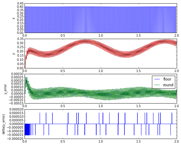

Here we have a pulse-width-modulated waveform going through a low-pass filter with time constant of \( \Delta t/\alpha = 0.2 \mathrm{s} \). Each of the fixed-point implementations is a good approximation to the floating-point implementation, typically within 0.0001 = 6.5 counts of output; the error between the two implementations is mostly zero within sporadic values of ±0.000015 = 1 count of output.

That’s just one anecdotal example, but you get the point.

Other algorithms like a Fast Fourier Transform, or a Kalman filter, or an IIR filter with a large number of taps, may be more sensitive to the effects of truncation vs. rounding, but in those cases if you’re using fixed-point arithmetic you should be studying your implementation very carefully to ensure that it’s doing the right thing, and the issue of rounding rather than truncation is only one of several important concerns, including overflow, scaling, and limit cycles.

Wrapup

You can reduce the numerical errors in your embedded system by rounding instead of using bitwise truncation (right-shifts) in fixed-point arithmetic. For runtime arithmetic, it may cost a few extra instruction cycles for each operation, however, and the decrease in error is often very small compared to other sources of error in the analog domain. So in many cases rounding at runtime may not be worth the effort.

Happy Thanksgiving!

© 2016 Jason M. Sachs, all rights reserved.

Sign in