Linear Feedback Shift Registers for the Uninitiated, Part XII: Spread-Spectrum Fundamentals

Last time we looked at the use of LFSRs for pseudorandom number generation, or PRNG, and saw two things:

• the use of LFSR state for PRNG has undesirable serial correlation and frequency-domain properties
• the use of single bits of LFSR output has good frequency-domain properties, and its autocorrelation values are so close to zero that they are actually better than a statistically random bit stream

The unusually-good correlation properties of an LFSR output bit stream make it possible to distinguish LFSR output from that of a “perfect” generator of random bits; while this is undesirable in some applications that need a source of statistically-random bits, it is ideal for other applications, which we will be describing next.

In this and the next few articles, we will be discussing spread-spectrum techniques, which is where LFSRs really excel.

Note: I will caution the reader that I have no professional experience with applications of communication theory — unless you count CRCs and COBS, and neither of those are hardcore theoretical topics. So some experienced readers may notice discrepancies between the examples in these articles and what is used in real-world communications systems. I would appreciate it if you bring any such discrepancies to my attention so I can attempt to fix them. In these articles, however, I am less concerned with getting the practical details perfect than with trying to explain the underlying concepts.

Spread-Spectrum in a Nutshell

The essence of spread-spectrum techniques is to take some signal \( x(t) \) of energy \( E \) that occupies a bandwidth \( B \) and encode it evenly within a bandwidth \( K_S B \) as a new signal \( x_S(t) \) using some kind of reversible operation. The value \( K_S > 1 \) is the spreading factor or spreading ratio. There are two major advantages of this approach:

• it allows the power spectral density \( E/B \) of the original signal to be reduced to \( E/K_S B \)
• such an encoding is less sensitive to additive disturbance signals \( d(t) \)

A receiver can reverse the process by “despreading” the raw received signal \( x_S(t) + d(t) \) and then filtering the resulting signal within bandwidth \( B \) to attempt to recover the original signal \( x(t) \).

There are several techniques for spread-spectrum; the two most common are frequency-hopping and direct-sequence spread spectrum (DSSS). This article focuses on DSSS.

Fourier Transforms for the Uninitiated

It occurs to me that some readers may not be familiar with Fourier transforms; I included some graphs in the last article that were frequency spectra, and these may be jumping the gun. So here’s a 10-minute introduction.

Suppose we have a sine wave \( x(t) = \cos (\omega t - \phi) \). There are a pair of mathematical identities based on Euler’s formula \( e^{j\theta} = \cos \theta + j\sin \theta \), that relate \( \cos \theta \) and \( \sin \theta \) to complex exponentials:

$$\begin{align} \cos\theta &= \frac{e^{j\theta} + e^{-j\theta}}{2} \cr \sin\theta &= \frac{e^{j\theta} - e^{-j\theta}}{2j} \end{align}$$

So we can write \( \cos \theta \) and \( \sin\theta \) as sums of complex exponentials. Do the math and you can figure it out for any phase angle:

$$\begin{align} \cos(\theta - \phi) &= \frac{e^{-j\phi}}{2}e^{j\theta} + \frac{e^{j\phi}}{2}e^{-j\theta} \end{align}$$

The mathematician and physicist Jean-Baptiste Joseph Fourier showed that any periodic function could be decomposed into a weighted sum of sine waves (and therefore as a weighted sum of complex exponentials); the Fourier transform is a mathematical technique that does this. The symbolic Fourier transform, like that of the Laplace transform, is a method of turning eager young students into despondent refugees from a life of mathematical study, for example by making them memorize all sorts of tables where a rectangular waveform is transformed into a sinc function, and a triangle wave is \( \frac{8}{\pi^2}\sum\limits_{n\ {\rm odd}}\frac{(-1)^{(n-1)/2}}{n^2} \sin \frac{n\pi x}{L} \), and so on. Aside from tests in university classes, you can look that stuff up if you need it; otherwise you may go mad. Don’t worry about it. The numeric Fourier transform, on the other hand, is incredibly useful; you just take any periodic waveform with \( N \) discrete-time samples \( x[k] \) taken at time intervals \( \Delta t \), and plug it into the Discrete Fourier Transform (DFT) formula:

$$ X [k] = \sum\limits _ {i=0} ^ {N-1} x[i] e^{-2\pi jik/N}$$

In go the time-domain samples \( x[k] \). Out come the frequency-domain coefficients \( X[k] \); these are measured in steps \( \Delta f = \frac{1}{N\Delta t} \). In practice, a Fast Fourier Transform (FFT) is usually used, which is algebraically identical but uses a divide-and-conquer approach to compute in \( O(N \log N) \) time rather than the \( O(N^2) \) that you get from evaluating the DFT directly. The time-domain samples are usually real-valued (as opposed to complex-valued with nonzero imaginary components), and this causes the frequency-domain coefficients to have some symmetric properties.

Let’s go through some examples using np.fft.fft to compute the FFT; here’s a 32-point cosine waveform:

%matplotlib inline
import numpy as np
import matplotlib.pyplot as plt
pi = np.pi

def show_fft(x, t=None, fig=None, style='-', 
             hide_upper_half=False, upper_half_as_negative=False,
             dbref=None, **kwargs):
    if fig is None:
        fig = plt.figure()
    N = len(x)
    
    ylim = kwargs.pop('ylim',None)
    freq_only = kwargs.pop('freq_only',False)

    if t is None:
        # support for pandas Series objects
        try:
            t = x.index
        except AttributeError:
            # fallback
            t = np.arange(N)
    if freq_only:
        ax_time = None
        ax_freq = fig.add_subplot(1,1,1)
    else:
        ax_time = fig.add_subplot(2,1,1)
        ax_freq = fig.add_subplot(2,1,2)
    X = np.fft.fft(x)
    
    if not isinstance(style, basestring) and len(style) == 2:
        tstyle, fstyle = style
    else:
        tstyle = fstyle = style
        
    
    if ylim is None:
        xmin = min(x)
        xmax = max(x)
        xspan = xmax-xmin
        ylim = (xmin-xspan*0.05, xmax+xspan*0.05)
    
    if not freq_only:
        ax_time.plot(t,x,tstyle,**kwargs)
        ax_time.set_xlim(min(t),max(t))
        ax_time.set_ylim(ylim)

    delta_t = t[-1]-t[0]  # this assumes equal spacing....
    df = 1/delta_t
    f = np.arange(N)*df
    if upper_half_as_negative:
        f[f/df>N/2] -= N*df
    if dbref is None:
        ax_freq.plot(f,np.abs(X),fstyle, **kwargs)
        ax_freq.set_ylim(0,np.abs(X).max()*1.05)
    else:
        ax_freq.plot(f,20*np.log10(np.abs(X)*1.0/dbref),fstyle, **kwargs)
        ax_freq.set_ylim(-120,20)
    if hide_upper_half:
        ax_freq.set_xlim(0,N*df/2)
    elif upper_half_as_negative:
        ax_freq.set_xlim(-N*df/2,N*df/2)
    else:
        ax_freq.set_xlim(0,N*df)

    return ax_time, ax_freq
    
N = 32
t = np.arange(N)*1.0/N
ax_time, ax_freq = show_fft(np.cos(2*pi*t), t, style=('.-','.'))
ax_time.set_ylabel('x(t)')
ax_time.set_xlabel('t')
ax_freq.set_ylabel('X(f)')
ax_freq.set_xlabel('f');

The top graph is the time-domain waveform \( x(t) = \cos 2\pi t \) sampled at \( N=32 \) subintervals; the bottom graph is the complex amplitude of the frequency domain \( X(f) \). For an integer number of periods \( P \) of a pure sine wave, the Fourier transform is zero except at two points: \( P \) and \( N-P \). Here we have one period, so the only nonzero coefficients of the Fourier transform are at \( f=1 \) and \( f=31 \). The amplitude is kind of funny; it’s 16, which is half the number of samples. You’d think, “Hey, the sine wave has amplitude 1, why doesn’t the frequency-domain component have amplitude 1? Why is it 16?” This is an artifact of the way the DFT is defined, and there are different definitions which can be used. Don’t worry about the amplitude in absolute terms; it’s just going to tell us the relative content at various frequencies. We only plot the complex amplitude here, which means we throw away phase information. Diehard DSP gurus will probably tell me that there’s some useful way to show phase information, but I don’t know of any, and when I use FFTs I usually just care about the amplitude, not the phase.

For real-valued time-domain waveforms, the upper half of the FFT is always symmetric with the lower half. This is kind of confusing, but there are a few ways of thinking about it. One is that the upper half of the FFT is really showing you negative frequencies (remember, \( \cos \omega t = \frac{e^{j\omega t} + e^{-j\omega t}}{2} \)), and it just wraps around in index like a circular buffer; we can display the FFT in a zero-centered way:

ax_time, ax_freq = show_fft(np.cos(2*pi*t), t, style=('.-','.'),
                            upper_half_as_negative=True)
ax_time.set_ylabel('x(t)')
ax_time.set_xlabel('t')
ax_freq.set_ylabel('X(f)')
ax_freq.set_xlabel('f');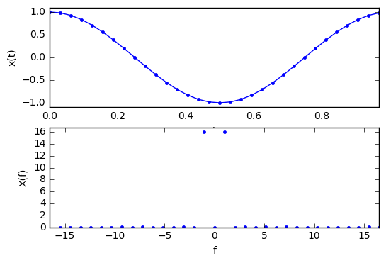

The other way to think about it is that we really do have a component at 31 times the fundamental frequency; this is an aliasing issue, and the Nyquist theorem says we can’t distinguish frequencies \( f \) from \( f_s-f \) where \( f_s \) is the sampling frequency — see for example the waveforms below — so the FFT will show both.

fig = plt.figure()
ax = fig.add_subplot(1,1,1)
ax.plot(t,np.cos(31*2*pi*t),'.')
t2 = np.arange(2000)*1.0/2000
ax.plot(t2,np.cos(31*2*pi*t2),'-')
ax.set_xlim(0,1);

In any case, because of the symmetry of real-valued waveforms, the upper half of the FFT doesn’t show any new information, so we’ll just hide it in all upcoming graphs.

def show_fft_real(x,t=None,**kwargs):
    ax_time, ax_freq = show_fft(x,t,hide_upper_half=True,**kwargs)
    if ax_time is not None:
        ax_time.set_ylabel('x(t)')
        ax_time.set_xlabel('t')
        ax_time.grid('on')

    if 'dbref' in kwargs and kwargs['dbref'] is not None:
        ax_freq.set_ylabel('X(f) (dB)')
    else:
        ax_freq.set_ylabel('X(f)')
    ax_freq.set_xlabel('f')
    ax_freq.grid('on')
    return ax_time, ax_freq

def cos2pi(t):
    return np.cos(2*pi*t)

show_fft_real(cos2pi(t),t,style=('.-','.'));

There. A sine wave at the fundamental frequency shows up as a single nonzero coefficient at \( f=1 \).

How about twice the fundamental frequency?

show_fft_real(cos2pi(2*t),t,style=('.-','.'));

One nonzero coefficient at twice the fundamental frequency. Piece of cake! Now let’s get into some more interesting stuff; let’s try a sum of sine waves:

show_fft_real(cos2pi(t) - cos2pi(3*t)/6,t,style=('.-','.'), ylim=[-1,1]);

That’s two nonzero components, one at the fundamental and one with 1/6 the amplitude at the third harmonic.

It is often easier to show FFT output on a decibel scale, showing the amplitudes relative to some standard level:

show_fft_real(cos2pi(t) - cos2pi(3*t)/6,t,style=('.-','.'), 
              dbref=32, ylim=[-1,1]);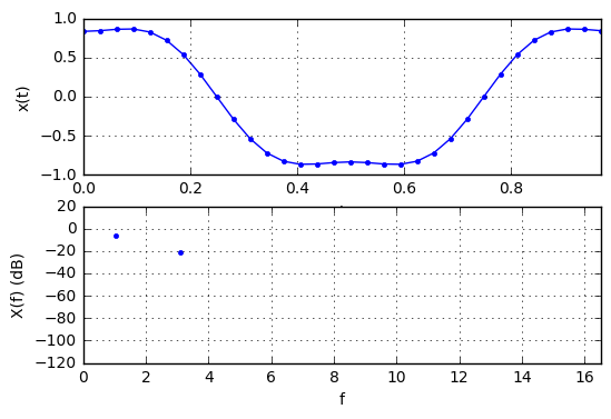

Here’s the spectrum of a flattened sine wave:

N=128
t = np.arange(N)*1.0/N
def smod(x,n):
    return (((x/n)+0.5)%1-0.5)*n
def flatcos(t):
    y = (cos2pi(t) - cos2pi(3*t)/6) / (np.sqrt(3)/2)
    y[abs(smod(t,1.0)) < 1.0/12] = 1
    y[abs(smod(t-0.5,1.0)) < 1.0/12] = -1
    return y
show_fft_real(flatcos(t),t,style=('.-','.'), dbref=N);

This is a variant of a raised cosine, and it has all sorts of harmonics, but they roll off fairly quickly (below -60dB for 9th harmonics and above), and we get a nice pleasing time-domain waveform.

We can also look at multiple periods of this waveform (or any other waveform, for that matter). Below is a graph showing \( N_1 = 10 \) periods; the nonzero amplitudes in frequency spectrum are exactly the same, but between each point of the frequency spectrum for 1 period, we’ve added another \( N_1-1 \) (=9) points with zero amplitude.

N1 = 10   # number of periods
N2 = 128  # number of samples per period
N = N1*N2
t = np.arange(N)*1.0/N2
show_fft_real(flatcos(t),t,style=('-','.'), dbref=N);

Okay, now we’ll do something a little more interesting and look at sending a bit pattern, in this case the ASCII encoding of the string “Hi” as a UART bitstream LSB-first, with one start bit, one stop bit, and two idle bits. We’ll look at the FFT of the resulting bitstream, with and without raised-cosine transitions:

import pandas as pd

def uart_bitstream(msg, Nsamp, idle_bits=2, smooth=True):
    """
    Generate UART waveforms with Nsamp samples per bit of a message.
    Assumes one start bit, one stop bit, two idle bits.
    """
    bitstream = []
    b_one  = np.ones(Nsamp)
    b_zero = b_one*-1
    bprev = 1
    if smooth:
        # construct some raised-cosine transitions
        t = np.arange(2.0*Nsamp)*0.5/Nsamp
        w = flatcos(t)
        b_one_to_zero = w[:Nsamp]
        b_zero_to_one = w[Nsamp:]
    def to_bitstream(msg):
        for c in msg:
            yield 0        # start bit
            c = ord(c)
            for bitnum in xrange(8):
                b = (c >> bitnum) & 1
                yield b
            yield 1        # stop bit
        for _ in xrange(idle_bits):
            yield 1
    for b in to_bitstream(msg):
        if smooth and bprev != b:
            # smooth transitions
            bitstream.append(b_zero_to_one if b == 1 else b_one_to_zero)
        else:
            bitstream.append(b_one if b == 1 else b_zero)
        bprev = b
    x = np.hstack(bitstream)
    t = np.arange(len(x))*1.0/Nsamp
    return pd.Series(x,t,name=msg)

def show_uart_bitstream_fft(msg, Nsamp=32, style='-', **kwargs):
    x = uart_bitstream(msg, Nsamp, **kwargs)
    axis_time, axis_freq = show_fft_real(x,dbref=len(x),style=style)
    axis_time.set_title('UART bitstream of message "%s"' % msg, fontsize=None)
    return axis_time, axis_freq

show_uart_bitstream_fft('Hi', Nsamp=16)
show_uart_bitstream_fft('Hi', Nsamp=16, smooth=False);

There are a few things to notice here.

• The bit period and fundamental frequency are both normalized to 1.0 here. So, for example, if we were using 100 bits per second, then the bit period would be 10ms and the fundamental frequency would be 100Hz, but the waveforms would look the same aside from scaling.
• Unlike all the waveforms we’ve looked at so far, these have mostly nonzero coefficients; these two spectra are kind of smeared out. That’s because they are rather nonperiodic in nature — although realize that the DFT and FFT treat their input as an infinitely-repeating signal.
• The frequency content in the interval \( f \in [0,1] \) represents the low-frequency content, and depends mostly on the bit pattern.
• The frequency content above \( f=1 \) represents the high-frequency content, and depends mostly on the transitioning between bits; with raised-cosine transitions, the frequency content drops by around 60dB (a voltage factor of 1000!) by \( f=4 \), whereas with sharp rectangular transitions the frequency content sticks around at high frequencies, like an unwanted relative who has stayed too long.

From here on out we’ll just use the raised-cosine waveform, and we’ll concentrate on the part of spectrum where \( f\leq 8 \); the higher frequency stuff is just more of the same, but attenuated. Below is the spectrum for the bitstream for the ASCII string “UUUUUUUU”. Why “U”? Because it has the ASCII code 85 = 0b01010101; in LSB-first form with start and stop bits it becomes 0101010101, and because of this nice alternating bit pattern it is often used in microcontrollers for automatic baud rate detection in UARTs.

axis_time, axis_freq = show_uart_bitstream_fft('UUUUUUUU')
axis_freq.set_xlim(0,8);

The spike at \( f=\frac{1}{2} \) is due to this strong regularity of alternating 0 and 1 bits; the only reason the spectrum doesn’t have complete gaps between these peaks is the idle time at the end of transmission, which tarnishes the periodicity of this waveform, and we get so-called spectral leakage between the peaks. If we get rid of the idle time then we’re left with a purely periodic waveform:

axis_time, axis_freq = show_uart_bitstream_fft('UUUUUUUU', 
                            idle_bits=0, style=('-','.'))
axis_freq.set_xlim(0,8);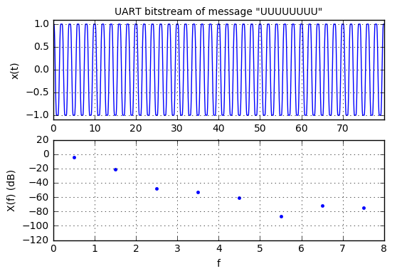

More erratic bit patterns lead to blurring in the spectrum:

axis_time, axis_freq = show_uart_bitstream_fft(
    'The quick brown fox jumps over the lazy dog')
axis_freq.set_xlim(0,8);

Here we have some smaller peaks which are most likely due to regularity at the byte level, and they should be at increments of \( f=\frac{1}{10} \) since there are 10 bits transmitted per byte (1 start bit + 8 data bits + 1 stop bit).

We’ll wrap up our spectral menagerie by looking at three more waveforms:

• white Gaussian noise from Python’s numpy.random.randn PRNG
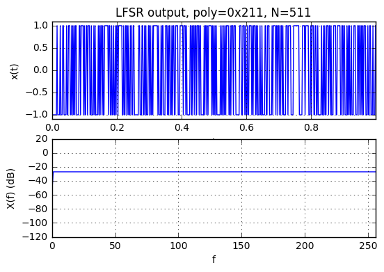
• white Bernoulli process noise (-1s and +1s) from the Python numpy.random.randint PRNG
• pseudonoise from an LFSR

N = 511
t = np.arange(N)*1.0/N
np.random.seed(1234)

xwhitenoise = np.random.randn(N)
ax_time, ax_freq = show_fft_real(xwhitenoise,t,dbref=N)
ax_time.set_title('White Gaussian noise, N=%d' % N)

xwhitebnoise = np.random.randint(0,2,size=(N,))*2-1
ax_time, ax_freq = show_fft_real(xwhitebnoise,t,dbref=N)
ax_time.set_title('White Bernoulli noise, N=%d' % N)

from libgf2.gf2 import GF2QuotientRing, checkPeriod
H211 = GF2QuotientRing(0x211)
assert checkPeriod(H211,511) == 511
def lfsr_output(field, initial_state=1, nbits=None):
    n = field.degree
    if nbits is None:
        nbits = (1 << n) - 1
    u = initial_state
    for _ in xrange(nbits):
        yield (u >> (n-1)) & 1
        u = field.lshiftraw1(u)
H211bits = np.array(list(lfsr_output(H211)))*2-1
ax_time, ax_freq = show_fft_real(H211bits,t,dbref=N)
ax_time.set_title('LFSR output, poly=0x%x, N=%d' 
                  % (H211.coeffs, len(H211bits)));

Both white noise spectra consist of irregular samples throughout their entire frequency range; they contain frequency content at all frequencies, low and high.

The LFSR output looks vaguely like white Bernoulli noise in the time domain, but in the frequency domain the spectrum is completely uniform in amplitude, which is something we looked at in the last article. Completely uniform! This is not an error! Over its entire period, the LFSR frequency components do this elaborate dance in the complex plane, with different phase angles but all having the same amplitude. As I mentioned last time, it’s better than a perfect PRNG. Too perfect for some applications, but as we’ll see next, it’s just right for spread-spectrum applications.

If we don’t sample the entire LFSR period, we get something that’s a little less regular:

H211bits = np.array(list(lfsr_output(H211, nbits=397)))*2-1
N = len(H211bits)
t = np.arange(N)*1.0/N
ax_time, ax_freq = show_fft_real(H211bits,t,dbref=N)
ax_time.set_title('LFSR output, poly=0x%x, N=%d' %
                  (H211.coeffs, N));

Anyway, now we’re ready to move back to the topic of spread-spectrum.

Spread-Spectrum Fundamentals

I mentioned there are several types of spread spectrum in common use; the two most common are frequency-hopping and direct-sequence spread spectrum. With both techniques, the idea is to conceal a narrow-band signal within a wider frequency range used for transmission.

For example, suppose I have some UART bitstream at 115200 baud. Because of the Nyquist theorem, the minimum bandwidth needed to transmit is twice this rate, or 230.4kHz. (We could reduce the bandwidth by using a multilevel modulation that uses a digital-to-analog converter to encode multiple bits at once — for example QAM or QPSK — but we’re not going to pursue those kind of schemes in this article.) If we just put out bits directly, they are centered at DC, and the required band is from -115200Hz to +115200Hz. But signals near DC don’t transmit via wireless, so unless we have a wire from point A to point B, this isn’t used. For RF transmission, we need to move the useful bandwidth to a higher frequency. This could be done with amplitude modulation (AM) or frequency modulation (FM) and use a different frequency range — but in any case, it will need at least 230.4kHz to reconstruct the original UART waveform, so we could use a band centered at 900MHz, from 899.885MHz to 900.115MHz.

Frequency-hopping

We could also use a wider range of frequencies. Frequency-hopping moves the band around over time, so for example, perhaps we transmit from 899.885MHz to 900.115MHz for one millisecond, then shift up to 904.885MHz to 905.115MHz for one millisecond, and shift to another band, and so on. It’s like a game of whack-a-mole — there’s a large pattern of holes on a table, and within any short time interval, the mole pops up from some specific hole in the table, but it moves around so much that to interfere with it, you need to target the entire set of holes. Apparently this — frequency hopping, not whack-a-mole — was invented by Nikola Tesla in a patent filed in 1900, although the language is kind of cryptic and Tesla never used the words spread-spectrum or frequency-hopping. An early non-cryptic explanation of spread-spectrum may be found in Jonathan Zenneck’s 1915 book Wireless Telegraphy, in which he describes:

185. Methods for Preserving Secrecy of Messages. — The fact that tuning does not in itself suffice to guard the secrecy of messages is a great disadvantage for many purposes (as in army and navy work).

The interception of messages by stations other than those called, can be prevented to some extent by telegraphing so rapidly that such relays as are customarily used will not respond and only specially trained operators will be able to read the messages in the telephone. Furthermore the apparatus can be so arranged that the wave-length is easily and rapidly changed and then vary the wave-length in accordance with a prearranged program perhaps automatically. This method makes it very difficult for an uncalled listener to tune his receiver to the rapid variations, but it is of no avail against untuned, highly sensitive receivers.

The more popularly-cited (but not the first) instance of early frequency-hopping was a patent filed in 1941 by Hedy Kiesler Markey (aka the actress Hedy Lamarr) and George Antheil covering secret communications by

a transmitting station including means for generating and transmitting carrier waves of a plurality of frequencies, a first elongated record strip having differently characterized, longitudinally disposed recordings thereon, record-actuated means selectively responsive to different ones of said recordings for determining the frequency of said carrier waves, means for moving said strip past said record-actuated means whereby the carrier wave frequency is changed from time to time in accordance with the recordings on said strip

and a similar receiving station with another “record strip” which could be operated in synchronization with the transmitting station “to maintain the receiver tuned to the carrier frequency of the transmitter.” In particular the record strips were envisioned as being like piano rolls with 88 rows, and one application was for “the remote control of dirigible craft, such as torpedoes.”

Lamarr and Antheil’s scheme utilized the whack-a-mole concept of frequency hopping, but did not describe the mathematically rigorous frequency-spreading aspect. It is harder to envision a signal modulated with a time-changing frequency, as a signal that is spread in overall bandwidth. Perhaps one can think of a time-lapse film of the mole moving so fast that it is a blur and appears to occupy all of the holes at once, although with a sort of ghostly transparency from being in each hole for only a short fraction of time.

At any rate, that’s the idea of frequency-hopping.

Direct-sequence spread-spectrum

The other commonly-used method of spread-spectrum is direct-sequence spread-spectrum, or DSSS. Suppose we consider our UART signal again, at 115200 baud. Each bit takes approximately 8.68μs to transmit. Now, we use some chipping signal \( s(t) \) consisting of values that are either \( +1 \) or \( -1 \), and is much faster, say at 16 times the bit rate, or 1.843MHz. The trick here is that we multiply the two to produce a spread waveform:

$$ x_s(t) = x(t)s(t) $$

Then at the receiving end, we take the received signal and multiply it by the same signal \( s(t) \), so that if there is no noise, \( x_r = x_s(t)s(t) = x(t)s^2(t) = x(t) \) because the chipping signal \( s(t) \) has the nice property that \( s^2(t) = 1 \). The faster bit rate of 16 times the bit rate is called the “chip rate”, and in this example the spreading factor \( K_S = 16 \).

Not any chipping signal will do; let’s use a square wave and see what happens:

msg = "Hi!"
fig = plt.figure()
x = uart_bitstream(msg, Nsamp=16, idle_bits=2)
s = np.hstack([[-1,-1,1,1]*(len(x)/4)])
xs = x*s
N = len(x)
show_fft_real(x, fig=fig, dbref=N)
ax_time, ax_freq = show_fft_real(xs, fig=fig,style=('.','-'),markersize=2.0,dbref=N);
ax_freq.legend(['$x(t)$','$x_s(t)$'],labelspacing=0);

Here the bandwidth has been shifted from DC to centered around \( 4f \) because we are multiplying by a periodic chipping sequence with period of 4 × the bit rate. The process of multiplying by a carrier frequency is called heterodyning, and it shifts the frequency but leaves its bandwidth unchanged. Now, however, let’s use an LFSR sequence:

def transmit_uart_dsss(msg, field, Nsamp, smooth=False, init_state=1):
    x = uart_bitstream(msg, Nsamp=Nsamp, idle_bits=2, smooth=smooth)
    N = len(x)
    s = np.array(list(lfsr_output(field,
                                  initial_state=init_state, 
                                  nbits=N)))*2-1
    return x, x*s

def show_dsss(msg, field, Nsamp=16, smooth=False):
    fig = plt.figure()
    x,xs = transmit_uart_dsss(msg, field, Nsamp=Nsamp, smooth=smooth)
    N = len(x)
    show_fft_real(x, fig=fig, dbref=N)
    ax_time, ax_freq = show_fft_real(xs, fig=fig,
                                     style=('.','-'),
                                     markersize=2.0, 
                                     dbref=N)
    ax_freq.legend(['$x(t)$','$x_s(t)$'],labelspacing=0,loc='best')

H1053 = GF2QuotientRing(0x1053)
assert checkPeriod(H1053,4095) == 4095
    
show_dsss("Hi!", field=H1053, Nsamp=16, smooth=True)

Here the reduced spectral density isn’t immediately obvious, but let’s crank up the spreading factor to 128:

show_dsss("Hi!", field=H1053, Nsamp=128, smooth=True)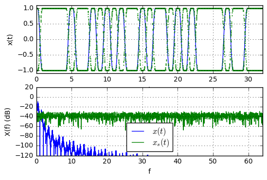

Now, in the real world, the DSSS modulation would happen before the edge-transition smoothing: just XOR the PN sequence with the desired data waveform. But the idea’s the same. We spread the spectrum out smoothly:

show_dsss("Hi!", field=H1053, Nsamp=128, smooth=False)

Now let’s model the receiver. We’re going to sidestep the problem of synchronizing the PN sequence as well as the bit boundaries, and pretend that our receiver already knows where both are, so that we can just use the following procedure:

• Take received waveform \( y(t) = x_{s}(t) + d(t) \) and multiply by the PN sequence \( s(t) \) to get \( x_r(t) = s(t)y(t) \)
• Integrate \( y(t) \) over each bit boundary
• Output a 1 if the integration result is positive, otherwise output a 0

In reality, the process of synchronizing PN at the receive side is nontrivial. It’s one thing to have a nice clean signal where we can look at bits and try to find a stretch of them where the data bit didn’t change, so that \( y(t) = s(t) \), and then just use state recovery techniques described in part VIII. But spread-spectrum is typically used in situations where the signal is buried among other competing signals, so some kind of fancy correlator gets used that figures out how to align things. (That’s my way of handwaving because I don’t really know an elegant way to get this done.) The UART side of things isn’t too fancy — just a state machine to sample multiple times per bit and synchronize to the data bit pattern by finding the start and stop bit — but since it’s not relevant to the concept at hand, I’ll just pretend we can skip that part.

With no noise, it’s kind of boring. Here’s an example:

def receive_uart_dsss(bitstream, field, Nsamp, initial_state=1,
                     return_raw_bits=False):
    N = len(bitstream)
    if field is None:
        xr = bitstream
    else:
        s = np.array(list(lfsr_output(field, 
                                      initial_state=initial_state,
                                      nbits=N)))*2-1
        xr = bitstream*s
    # Integrate over intervals:
    #   - cumsum for cumulative sum
    #   - decimate by Nsamp
    #   - take differences
    #   - skip first sample
    xbits = (xr.cumsum().iloc[::Nsamp].diff()/Nsamp).shift(-1).iloc[:-1]
    if return_raw_bits:
        return xbits
    #   - test whether positive or negative, convert to 0 or 1
    xbits = (xbits > 0).values*1
    # now take each stretch of 10 bits, 
    # grab the middle 8 to drop the start and stop bits,
    # and convert to an ASCII coded character 
    msg = ''
    for k in xrange(0,10*(len(xbits)//10),10):
        bits = xbits[k+1:k+9]
        ccode = sum(bits[j]*(1<<j) for j in xrange(8))
        msg += chr(ccode)
    return msg

def error_count(msg1, msg2):
    errors = 0
    for c1,c2 in zip(msg1, msg2):
        if c1 != c2:
            errors += 1
    return errors

def signal_energy(signal, t=None):
    if t is None:
        t = signal.index
    return np.trapz(signal**2, t)

def error_count_msg(msg1, msg2):
    err = error_count(msg1, msg2)
    return err, "%d errors out of %d bytes" % (err, len(msg1))
    
msg1 = '''"The time has come," the Walrus said,
"To talk of many things:
Of shoes---and ships---and sealing-wax---
Of cabbages---and kings---
And why the sea is boiling hot---
And whether pigs have wings."'''
x,xs = transmit_uart_dsss(msg1, H1053, Nsamp=128)
msgr = receive_uart_dsss(xs, H1053, Nsamp=128)
print msgr
print error_count_msg(msg1, msgr)[1]
print "signal energy:", signal_energy(x)

"The time has come," the Walrus said,
"To talk of many things:
Of shoes---and ships---and sealing-wax---
Of cabbages---and kings---
And why the sea is boiling hot---
And whether pigs have wings."
0 errors out of 195 bytes
signal energy: 1951.9921875

Round 1: Spread-spectrum vs. Noise

Now here’s the neat part; we’ll add some noise. It looks like Gaussian noise starts to cause some difficulties once we reach about a standard deviation of about 4-4.5 times the DSSS-modulated waveform. That’s a huge amount of noise! Here’s random noise with standard deviation of 4.7 times greater than the digital waveform:

np.random.seed(123)
disturbance1 = 4.7*np.random.randn(len(xs))
y1ss = xs + disturbance1
ndisp=160
plt.plot(y1ss[:ndisp])
plt.plot(xs[:ndisp])
plt.xlabel('bit index')
msgr = receive_uart_dsss(y1ss, H1053, Nsamp=128)
print msgr
print error_count_msg(msg1, msgr)[1]
def energy_msg(x, disturbance):
    Ex = signal_energy(x)
    Ed = signal_energy(disturbance, t=x.index)
    snr = 10*np.log10(Ex/Ed)
    msg = (
        "signal energy:      %7.1f\n"
       +"disturbance energy: %7.1f\n"
       +"SNR:                %7.1fdB") % (Ex, Ed, snr)
    return snr, msg
print energy_msg(xs, disturbance1)[1]

"The time has`come," the Walrus said,
"Po talk of many things:
Ofshoes---anD ships-�-aod sealin'-wax---
Od cabbages---and kings---
And why the sea is boiling hot---
And whataer pigs (ave!w�ngs."
13 errors out of 195 bytes
signal energy:       1952.0
disturbance energy: 42977.5
SNR:                  -13.4dB

In this and the following graphs, I’m only showing the first 160 bits so that it is a little bit easier to see — otherwise the full 1950 bits is one big blur.

The thing is, we can get about the same bit error rate without bothering to use spread-spectrum:

y1 = x + disturbance1
ndisp=160
msgr = receive_uart_dsss(y1, field=None, Nsamp=128)
plt.plot(y1[:ndisp])
plt.plot(x[:ndisp])
plt.xlabel('bit index')
print msgr
print error_count_msg(msg1, msgr)[1]
print energy_msg(x, disturbance1)[1]

"The time law come," the Walvus said,
"To ta�k of many thyngs:
Of sj�es---and ships---and sealing-wax---
Of cabbages---and0kings---
And why the sea is bgiling �/t---
And whgthws pigs have wings."
14 errors out of 195 bytes
signal energy:       1952.0
disturbance energy: 42977.5
SNR:                  -13.4dB

The noise immunity here comes from the fact that we take the average value over the 128 samples per bit, in which case the raw received waveform looks like this:

ndisp = 160
Nsamp=128
msgr = receive_uart_dsss(y1, field=None, Nsamp=Nsamp, return_raw_bits=True)
x0 = x.iloc[::Nsamp]            # original bit pattern (1 sample per bit)
# received bits and original +/- 1 bits are opposite sign
error_indices = np.argwhere(msgr*x0<0)[:,0]
ii = error_indices[error_indices<ndisp]
for w in [msgr,x0]:
    plt.plot(w[:ndisp],drawstyle='steps-post',linewidth=0.8)
plt.plot(ii+0.5, msgr[ii],'.')
plt.xlabel('bit index');

The averaged noise is just enough to flip a few of the received bits (highlighted with red dots in the graph above). With oversampling by a factor of \( N_a \) and averaging, we reduce the variance of the noise by a factor of \( N_a \), which is a reduction in standard deviation by a factor of \( \sqrt{N_a} \), or \( \sqrt{128} \approx 11.31 \) in this case, bringing the effective noise level to 4.7/11.31 = an expected standard deviation of 0.415 relative to the bit level. We can see that if we take a histogram:

from scipy.stats import norm

def show_error_histogram(err, bins=None, binsize=0.1):
    errmin = min(err)
    errmax = max(err)
    if bins is None:
        bins = np.arange(np.floor(errmin/binsize),
                         np.ceil(errmax/binsize))*binsize
    err.hist(bins=bins, label='histogram')
    sample_std = err.std()
    print "sample standard deviation of error:", sample_std

    norm_distribution = norm.pdf(bins/sample_std)
    A = len(err)/sum(norm_distribution)
    errx = np.arange(0,1,0.005)*(errmax-errmin) + errmin
    plt.plot(errx, A*norm.pdf(errx/sample_std),
             label='expected distribution')
    plt.xlabel('signal error (received-original)')
    plt.ylabel('number of samples')
    plt.legend(loc='best',fontsize=10,labelspacing=0)
show_error_histogram(x0-msgr,binsize=0.1)

sample standard deviation of error: 0.426599071579

Round 2: Spread-spectrum vs. Disturbance

What’s more interesting is if we add in a disturbance signal that is not noise, for example a frequency sweep:

from scipy.integrate import cumtrapz

t = x.index
p = 120.0
triwave = np.abs(4*((t/p - 0.5) % 1) - 2)-1
trapz = np.clip(1.1*triwave,-1,1)
freq = 5.5+4.5*trapz
angle = cumtrapz(freq, t, initial=0)
disturbance2 = pd.Series(2.2*np.sin(angle),t)
ndisp = 160
disturbance2[:ndisp].plot()
x[:ndisp].plot()
plt.xlabel('bit index');

Now let’s see how this affects reception of the message:

y2 = x + disturbance2
ndisp=160
msgr = receive_uart_dsss(y2, field=None, Nsamp=128)
plt.plot(y2[:ndisp])
plt.plot(x[:ndisp])
plt.xlabel('bit index')
print msgr
print error_count_msg(msg1, msgr)[1]
print energy_msg(x, disturbance2)[1]

#�he time �1s�come," t�9!�alrus sa�91�"To talk�3(many thi�
1*
Of shoew
9-and shipU
9-and sealU̹-wax---
OU��abbages--U��e kings--U��md why thU��ea is boiM��U hot---
A��Twhether p�NU have winfFV"
57 errors out of 195 bytes
signal energy:       1952.0
disturbance energy:  4723.7
SNR:                   -3.8dB

Almost one third of the received bytes have errors! Now let’s add the same disturbance to a spread-spectrum transmission of the same message:

y2ss = xs + disturbance2
ndisp=160
plt.plot(y2ss[:ndisp])
plt.plot(xs[:ndisp])
plt.xlabel('bit index')
msgr = receive_uart_dsss(y2ss, H1053, Nsamp=128)
print msgr
print error_count_msg(msg1, msgr)[1]
print energy_msg(xs, disturbance2)[1]

"The time has come," the Walrus said,
"To talk of many things:
Of shoes---and ships---and sealing-wax---
Of cabbages---and kings---
And why the sea is boiling hot---
And whether pigs have wings."
0 errors out of 195 bytes
signal energy:       1952.0
disturbance energy:  4723.7
SNR:                   -3.8dB

No errors! What’s going on?

The frequency-sweep disturbance is concentrated at the low end of the spectrum. For the bitstream transmitted without spread-spectrum, this disturbance occupies much of the same signal. For the bitstream transmitted with spread-spectrum, this disturbance contaminates only a small portion of the transmitted frequency spectrum:

fig = plt.figure()
N = len(x0)
show_fft_real(xs, fig=fig, dbref=N,freq_only=True)
_, ax_freq = show_fft_real(disturbance2, fig=fig,dbref=N,freq_only=True)
ax_freq.set_ylim(-90,40)
ax_freq.legend(['DSSS-encoded signal','disturbance2'],fontsize=10)
ax_freq.set_title('Frequency spectra of raw received signal');

When we multiply by the chipping sequence,

• the DSSS-encoded signal is transformed back to the original bitstream, occupying only the low-frequency bandwidth
• the disturbance is transformed into a scrambled disturbance over the entire frequency range

The graph below shows this, and towards the lower end, the original signal peeks up above the noise of the scrambled disturbance:

N = len(x0)
s = np.array(list(lfsr_output(field=H1053, nbits=len(xs))))*2-1

x_processed = xs*s
disturbance2_processed = disturbance2*s

fig = plt.figure()
show_fft_real(x_processed, fig=fig, dbref=N,freq_only=True)
_, ax_freq = show_fft_real(disturbance2_processed, fig=fig,
                           dbref=N,freq_only=True)
ax_freq.legend(['Original signal','scrambled disturbance2'],
               fontsize=10,loc='lower left')
ax_freq.set_ylim(-90,40)
ax_freq.set_title('Frequency spectra of despread signal');

In the real world we don’t receive our signal and noise separately; they are added together, but you can still see the signal peeking up above the noise at the low end:

fig = plt.figure()
_, ax_freq = show_fft_real(y2ss * s, fig=fig, dbref=N,freq_only=True)
ax_freq.set_ylim(-90,40)
ax_freq.set_title('Frequency spectra of despread signal');

After filtering, the signal does have some residual error, but not enough to flip a bit:

msgr = receive_uart_dsss(y2ss, field=H1053, Nsamp=Nsamp, return_raw_bits=True)
msgr[:ndisp].plot(drawstyle='steps-post')
x0[:ndisp].plot(drawstyle='steps-post')
plt.xlabel('bit index');

show_error_histogram(x0-msgr,binsize=0.02)

sample standard deviation of error: 0.140077253704

We should be able to double or maybe even triple the disturbance level and still avoid bit errors:

def signal_energy(signal, t=None):
    if t is None:
        t = signal.index
    return np.trapz(signal**2, t)

snrlist = []
for kd in np.arange(2.0,4.01,0.2):
    disturbance3 = kd*disturbance2
    y2ss2 = xs + disturbance3
    msgr = receive_uart_dsss(y2ss2, H1053, Nsamp=128)
    errct, errmsg = error_count_msg(msg1, msgr)
    snr, emsg = energy_msg(xs, disturbance3)
    snrlist.append((1.0*errct/len(msg1),snr))
    if errct < 30:
        # we don't need to see results for lots of errors
        print "disturbance amplitude: %.2f" % np.abs(disturbance3).max()
        print msgr
        print errmsg
        print emsg
        print ""

disturbance amplitude: 4.40
"The time has come," the Walrus said,
"To talk of many things:
Of shoes---and ships---and sealing-wax---
Of cabbages---and kings---
And why the sea is boiling hot---
And whether pigs have wings."
0 errors out of 195 bytes
signal energy:       1952.0
disturbance energy: 18894.7
SNR:                   -9.9dB

disturbance amplitude: 4.84
"The time has come," the Walrus said,
"To talk of many things:
Of shoes---and ships---and sealing-wax---
Of cabbages---and kings---
And why the sea is boiling hot---
And whether pigs have wings."
0 errors out of 195 bytes
signal energy:       1952.0
disturbance energy: 22862.6
SNR:                  -10.7dB

disturbance amplitude: 5.28
"The time hqs come," the Walrus said,
"To talk of many things:
Of shoes---and ships---and sealing-wax---
Of cabbages---and kings---
And why the sea is boiling hot---
And whether pigs have wings."
1 errors out of 195 bytes
signal energy:       1952.0
disturbance energy: 27208.4
SNR:                  -11.4dB

disturbance amplitude: 5.72
"The time hq� come," the Walrus said,
"To talk of many things:
Of shoes---and ships---and sealing-wax---
Of cabbages---and kings---
And why the sea is boiling hot---
And whether pigs have wings."
2 errors out of 195 bytes
signal energy:       1952.0
disturbance energy: 31932.1
SNR:                  -12.1dB

disturbance amplitude: 6.16
"The time hq� come," the Walrus said,
"To talk of many things:
Of sioes---and ships---and sealing-wax---
Of cabbages---and kings---
And why the sea is boiling hot---
And whether pigs have wings."
3 errors out of 195 bytes
signal energy:       1952.0
disturbance energy: 37033.6
SNR:                  -12.8dB

disturbance amplitude: 6.60
"The time hq� come," the Walrus said,
"To talk of many things:
Of sioes---and ships---and sealing-wax---
Of cabbages---and kings---
And why the sea!is boiling hot---
And whether pigs have wings."
4 errors out of 195 bytes
signal energy:       1952.0
disturbance energy: 42513.1
SNR:                  -13.4dB

disturbance amplitude: 7.04
"The time hq� come." the Walrus siid,
"To talk of many things:
Of sioes---anl ships---and sealing-wa�---
Of cabbages---and kings---
And why the seq!�s boiling hot---
And whether pigs have whngs."
11 errors out of 195 bytes
signal energy:       1952.0
disturbance energy: 48370.5
SNR:                  -13.9dB

disturbance amplitude: 7.48
"Tle time0hq� come." the Walrus siid,
"To talk of many things:
Of sioes-)-anl ships---and sealing-wa�--=
Of c`bbages---and kings--=
And why the seq!�s boilinf hot%--
And whether rigs hafe whngs."
21 errors out of 195 bytes
signal energy:       1952.0
disturbance energy: 54605.7
SNR:                  -14.5dB

The signal-to-noise ratio (SNR) at which we start to see errors is no coincidence; with our filtering method of averaging each 128 samples, this reduces the energy of white noise by \( 10 \log_{10} 128 \approx 21 \)dB for an SNR gain of 21dB. White Gaussian noise with unit amplitude has a standard deviation of 1, so it’s pretty easy to figure out a bit rate error as the fraction of samples that exceed ±1 for some large number of normally-distributed pseudorandom samples:

from scipy.stats import norm

np.random.seed(123)
npoints = 1000*1000
unit_noise = np.random.randn(npoints)
def db_to_amplitude(db):
    return 10**(db/20.0)
dbmin = -5
dbmax = 15
dbrange =  np.arange(dbmin,dbmax)
dbrangefine = np.linspace(dbmin,dbmax,1000)
bit_error_rate = [np.count_nonzero((unit_noise
                                    /db_to_amplitude(db)>1) )
                  *1.0/npoints  for db in dbrange]
walrus_data = np.array(snrlist)
walrus_bit_error_rate = walrus_data[:,0]
walrus_snr = walrus_data[:,1] + 10*np.log10(128) 
      # account for 128:1 averaging
fig = plt.figure()
ax = fig.add_subplot(1,1,1)
ax.semilogy(dbrangefine, norm.cdf(-db_to_amplitude(dbrangefine)),
            '-', linewidth=0.5)
ax.semilogy(dbrange, bit_error_rate, '.')
ax.semilogy(walrus_snr, walrus_bit_error_rate,'x')
ax.grid('on')
ax.set_xlim(dbmin,dbmax)
ax.set_xlabel('SNR (dB)')
ax.set_ylabel('Bit error rate')
ax.legend(['Theoretical curve',
           'Random samples of Gaussian',
           'Walrus spread-spectrum data'],
         fontsize=10, loc='lower left',
         labelspacing=0);

This is a pretty typical graph for bit error rate. At low values of SNR there are lots of errors; with higher values of SNR the probability of error rapidly drops, and it’s hard to verify empirically without running into Black Swan effects, which is why that green dot at 13dB is below the curve and there are no dots beyond it. The experimental data for our spread-spectrum data is a little bit higher than for independent random Gaussian samples — and perhaps that’s because the simple boxcar averaging of 128 values isn’t a very good filter to use; maybe we should be using a filter with a sharper cutoff.

The theoretical curve here is based on the cumulative distribution function (CDF) of a Gaussian distribution; we’re basically looking at area of one tail of the probability distribution function (PDF) where outlying data is greater than a particular threshold, namely \( Q(a) = \Phi(-a) \) for some number of standard deviations \( a = 10^{\rm SNR/20} \) for SNR in dB. (\( Q(x) \) is the Q-function in statistics, found on some scientific calculators, and represents the probability that a unit Gaussian random variable is greater than \( x \). The astute reader will also note that sometimes when converting between dB and a raw signal, we use 20dB/decade and other times 10dB/decade; the conversion factor is 20dB/decade when dealing with amplitude, and 10dB/decade when dealing with power and energy, which are proportional to amplitude squared.)

(Note: originally this article used both tails of the PDF, which is incorrect. If we have a bit sequence consisting of \( \pm A \), then when the signal is \( +A \), a positive error will not result in a decoded bit flip, whereas a negative error will cause a decoded bit flip only if that error is below \( -A \). Similarly, when the signal is \( -A \), a negative error will not result in a decoded bit flip, whereas a positive error will cause a decoded bit flip only if that error is above \( +A \). Both tails are involved, but only one at a time depending on what the signal is, so the average error rate is \( Q(a) \).)

x = np.arange(-5,5,0.001)
fig=plt.figure(figsize=(6,1.5))
ax=fig.add_subplot(1,1,1)
y = norm.pdf(x)
a = 1.8
ax.plot(x,y)
for whichtail in [-1,1]:
    xtail = x[x*whichtail > a]
    ytail = norm.pdf(xtail)
    ax.fill_between(xtail,0,ytail,facecolor='green',edgecolor='none')
ax.set_xlim(-5,5)
ax.set_xticks([-a,a]);
ax.set_yticks([])
ax.set_xticklabels(['-a','a']);
ax.set_title('Tails of a Gaussian PDF');

Round 3: Sharing is Caring — Spread-spectrum vs. Spread-Spectrum

So far we’ve looked at only one transmitter; part of the benefits of spread-spectrum is that it is possible for more than one transmitter to share bandwidth; we just have to use a non-interfering modulation sequence. Shown below is one example; we’ll encode the Walrus and Carpenter excerpt using DSSS with one LFSR output sequence, and encode part of Jabberwocky using DSSS with another LFSR output sequence, and add them together, then decode both from the same transmitted signal:

msg2 = '''\'Twas brillig, and the slithy toves
Did gyre and gimble in the wabe:
All mimsy were the borogoves,
And the mome raths outgrabe. 

"Beware the Jabberwock, my son!
The jaws that bite, the claws that catch!
Beware the Jubjub bird, and shun
The frumious Bandersnatch!'''

# pad msg1 so they have the same length
msg1 += ' '*(len(msg2) - len(msg1))

Nsamp=128
x1,xs1 = transmit_uart_dsss(msg1, H1053, Nsamp=Nsamp)
# offset LFSR sequence by about half the period
state2 = H1053.lshiftraw(1,2048)
x2,xs2 = transmit_uart_dsss(msg2, H1053, Nsamp=Nsamp, 
                            init_state=state2)

# add both sequences
y = xs1 + xs2

msgr1 = receive_uart_dsss(y, H1053, Nsamp=Nsamp, 
                          initial_state=1)
print msgr1
print error_count_msg(msg1, msgr1)[1]
print ""

msgr2 = receive_uart_dsss(y, H1053, Nsamp=Nsamp, 
                          initial_state=state2)
print msgr2
print error_count_msg(msg2, msgr2)[1]

"The time has come," the Walrus said,
"To talk of many things:
Of shoes---and ships---and sealing-wax---
Of cabbages---and kings---
And why the sea is boiling hot---
And whether pigs have wings."                                                                    
0 errors out of 263 bytes

'Twas brillig, and the slithy toves
Did gyre and gimble in the wabe:
All mimsy were the borogoves,
And the mome raths outgrabe. 

"Beware the Jabberwock, my son!
The jaws that bite, the claws that catch!
Beware the Jubjub bird, and shun
The frumious Bandersnatch!
0 errors out of 263 bytes

No errors! This is because spread-spectrum makes each of the signals look like noise to the other one; here’s the received spectrum as seen by receiver 2:

s = np.array(list(lfsr_output(field=H1053, 
                              initial_state=state2,
                              nbits=len(xs1))))*2-1

fig = plt.figure()
_, ax_freq = show_fft_real(y * s, fig=fig, 
                           dbref=len(xs1)/Nsamp,
                           freq_only=True)
ax_freq.set_ylim(-90,40)
ax_freq.set_title('Frequency spectra of despread signal');

You can see the spectrum of message 2 peeking up above the “noise” of message 1 after it’s been despread by the LFSR sequence used for receiving message 2.

There is a catch here; we have to keep the chipping sequences uncorrelated. One way to do this is use the same LFSR output sequence, shifted in time — as we did in this contrived example — but that’s not really practical, because it would require time synchronization among all transmitters. Without such time synchronization, there’s a small chance that two transmitters would use a chipping sequence which is close enough that they would interfere, and the birthday paradox says that this goes up as the square of the number of transmitters. In practice, other methods are used, and we’ll talk about one of them (Gold codes) in an upcoming article.

Where do we go from here? For basic direct-sequence spread-spectrum concepts, that’s about it. Next time we’ll be looking at applications of spread-spectrum for system identification.

Wrapup

With so many graphs — I think this is the article that sets the record — what we showed may be a little bit hazy. Here’s a summary:

• Direct-sequence spread spectrum (DSSS) is implemented by modulating a data bitstream with a chipping signal with amplitude ±1 and a bit rate that is some factor \( K_S \) greater than the bandwidth of the data bitstream.

  • With a digital data bitstream, XOR is used
  • With an analog data bitstream, multiplication is used
  • \( K_S \) is the spreading factor or spreading ratio.
  • LFSR output bit sequences are sufficient for a chipping signal
  • The chipping signal doesn’t have to be that of an LFSR; any sequence with amplitude ±1 and reasonably flat frequency spectrum can be used, although LFSR output sequences are very convenient

• DSSS demodulation reverses the process

  • The same chipping sequence must be used in a synchronized manner to demodulate the received bitstream
  • DSSS demodulation essentially scrambles the spectrum of any disturbance
  • Low-pass filtering to include all of the original signal bandwidth is used, to filter out noise or disturbance

• DSSS provides no benefits in reducing the disturbance of wideband noise that covers the full spectrum of the modulated sequence (see Round 1)

• DSSS provides increased noise immunity to narrow-band disturbances, by spreading their energy (during demodulation) over the entire bandwidth of the modulated signal (see Round 2)
• DSSS can allow multiple transmitters to share transmission bandwidth when using chipping signals that are uncorrelated (see Round 3)

References

• Jan Meel, Spread Spectrum (SS) — introduction, De Nayer Instituut, Sint-Katelijne-Waver, Belgium, 1999.

• Raymond L. Pickholtz, Donald L. Schilling, Laurence B. Milstein, Theory of Spread-Spectrum Communications — A Tutorial, IEEE Transactions on Communications, vol. 30, no. 5, pp. 855-884, May 1982.

Both of these are excellent introductory references; of the two, Jan Meel’s has more pretty pictures, and Pickholtz et al goes deeper into the theory.

© 2017 Jason M. Sachs, all rights reserved.

Sign in