• Audio DSP
• Matlab
• Probability

Introduction

Hello! This is my first post on dsprelated.com. I have a blog that I run on my website, http://www.christianyostdsp.com. In order to engage with the larger DSP community, I'd like to occasionally post my more engineering heavy writing here and get your thoughts.

Today we will look at the phase vocoder from a different angle by bringing some probability into the discussion. This is the first part in a short series. Future posts will expand further upon the ideas introduced here. After learning the basic PV idea, we might wonder what would warrant an investigation into improvements. Let’s start by reminding ourselves of the informal phase vocoder algorithm description: 

When we measure how much the phase changed in our current frame from its previous frame, we are looking at how far each 3D-complex sinusoid turned over the analysis time period. Then we use this information to estimate how much the corkscrew will probably turn over the next analysis time period. Here it is important to note that the phase vocoder creates an approximation to the hypothetical signal we are trying to create. 

We see here that the next state of the classic phase vocoder is completely dependent on its current state. Processes that behave in such a way are known as Markov processes. Wikipedia gives us the following definition [1]: 

A stochastic process has the Markov property if the conditional probability distribution of future states of the process (conditional on both past and present states) depends only upon the present state, not on the sequence of events that preceded it. A process with this property is called a Markov process.

Now most people wouldn’t describe the phase vocoder as “stochastic”, and the signals fed into the PV certainly aren’t random, however, from the point of view of the computer, they can appear to be. In one sense, statistics is the tool people created to deal with a set of possibilities, which are not necessarily random. We can think about statistics in card gambling. The order of cards in a deck isn’t random. It is completely determined by iterations of different shuffling patterns from an initial, constant state, that summed up until the present will tell you their order. If the shuffling patterns are the same, the resultant order will be the same no matter the deck. While this process isn’t random, it is as good as random to us, because there is no way we could know all the shuffling patterns that have affected the deck. Even if you knew all shuffles but one, you couldn’t know the current order! Because of this, probability is used to get a sense of the general structure of a card deck. 

Something similar can be said about musical signals, except we are the shuffling patterns, and the computer is us. We know everything that happens in the signal we feed into the phase vocoder, and the computer doesn’t. And if we go through some lengthy scheme to program every feature in the signal, we have completely sacrificed real-time control, which is perhaps the most valuable feature of the phase vocoder. Like how seeing three “face” cards on the table let’s you know that face cards are much less likely to be drawn, knowing that a sinusoidal component is in a certain bin hints that it is much less likely to move to some frequency bin 10,000 Hz away. This gives us some sense of the sinusoidal structure of the signal. 

Statistical Considerations 

So how would we construct a general structure for a musical signal? How can we determine if a structure exists at all? Well it seems like some locations are far more likely a destination for a given frequency than others. And if we see that there is at least one location less preferred than another, by induction perhaps we can infer that there exists some order of location preference that we could call the signal’s sinusoidal structure. Now this obviously doesn’t suffice as a rigorous mathematical proof, but it does tell us that investigation into the time-frequency information of a signal is likely to produce some outline of a structure within the signal. Many DSP engineers, some of whom are mentioned in post 3, have approached the phase vocoder with some signal sinusoidal structure in mind. I spent most of 2018 investigating these solutions and designing real-time implementations during my undergraduate senior project. Here I’d like to take a step back and show why so many people have looked into these solutions in the first place. The result should be some quantitative base to rest our intuitions on. Using the idea of a Markov Chain, we will tease out a general structure that musical signals have. It is exactly structures like this one which engineers have used to guide their improved phase vocoder algorithms. 

Since the classic phase vocoder’s future state depends entirely on the current one, and the signal it’s operating on isn’t known to the computer, we can say it behaves like a Markov Chain. This means there exists a transition graph which expresses the next location of a sinusoid in a given bin as a probability. Below, the Y-axis represents the current location of a sinusoid, and the X-axis represents the next location of a sinusoid. Table 1 illustrates the structure which the phase vocoder assumes. 

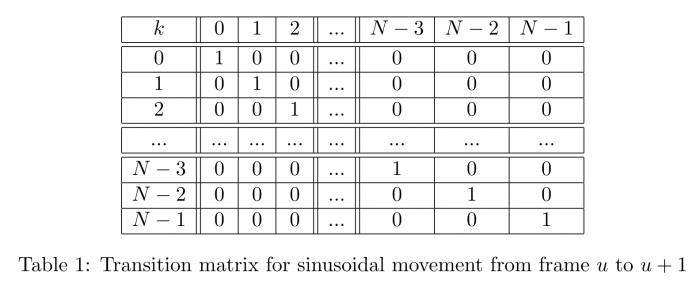
This doesn’t seem like an accurate view of an input signal, so let’s start an investigation into some properties of a signal to see if we can create a better transition graph. Since we are working with probability and statistics, let’s start with some elementary equations that we will use later on in our calculations.

\begin{equation*}\label{mean} \bar{x} = \frac{\sum_{i=0}^{N-1}x_{i}}{N} \end{equation*} \begin{equation*}\label{cov} Cov(X,Y) = \frac{\sum_{i=0}^{N-1}(x_{i}-\bar{x})(y_{i}-\bar{y})}{N} \end{equation*} \begin{equation*}\label{sd} \sigma(X) = \sqrt{\frac{1}{N}\sum_{i=0}^{N-1}(x_{i}-\bar{x})^{2}} \end{equation*} \begin{equation*}\label{covxx} Cov(X,X) = \frac{\sum_{i=0}^{N-1}(x_{i}-\bar{x})^{2}}{N} = (\sigma(x))^{2} \end{equation*}

Consider the amplitude envelopes of two adjacent frequency bins. Suppose that a single sinusoidal component in some mixture occupies each frequency bin at adjacent time points. In such a case we would expect to see a similar change in the amplitude envelope of each frequency as the sinusoid moves from one bin to the other. However, the amplitude difference in the bin it is coming from should be opposite of the change in amplitude of the bin it is going to. Figure 1 illustrate this behavior.

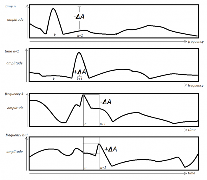
So if there is a change in amplitude in a given frequency bin, and we observe a similar amplitude change in another frequency bin, that amplitude difference could be coming from the same source, in other words sinusoidal movement. In order to get a sense of such sinusoidal movement, for each frequency bin we will calculate the covariance and correlation between its amplitude difference envelope and the amplitude difference envelope of every other frequency bin. The results will be plotted in an $N/2 \times N/2$ matrix. We choose $N/2$ because the second half of the spectrum is just a mirror of the first. Because $Cor(X,X) = 1$, we expect there should be a diagonal line across the matrix, similar to the one the phase vocoder assumes.

Implementation 

The linked MATLAB code will calculate this matrix. It starts by recording the spectrum of the signal, as well as the amplitude difference between two adjacent FFT frames both in principle value and as a change proportional to its previous amplitude. For each time point, we will calculate the mean amplitude difference and its standard deviation, again both in principle and proportional value. The frequency amplitude vs. time plots we looked at earlier will also be calculated. For each frequency bin we can see the mean and standard deviation of the amplitude and amplitude difference. Finally the script uses this information to calculate the covariance and correlation between frequency bins. A couple notes about the script and calculations: 

1. When calculating proportional change, we set a gate so that channels whose current and previous amplitude is below the gate are ignored. This is because many frequency bins have little to no energy, so small increases in energy show up as up to 25x’s increase in energy, when in reality it is an inaudible frequency component. 

2. From that data we calculate the mean absolute value difference as well as the standard deviation of that difference for a given frequency. The absolute value is a more desirable version of the difference. Because the signal starts and ends quietly, if we think about what the mean value theorem says, the average amplitude difference is actually zero. So by taking the absolute value, we see the average change each frequency experiences per frame. Additionally, both positive and negative changes in amplitude are signs of sinusoidal movement, as we saw above.

The input signal we will use will be 7 seconds of Bach’s Violin Sonata No. 1 in G minor [2]. This seems like a nice choice because it is only one voice, and has a fair amount of sinusoidal movement. The FFT size is N = 1024 and we will use a Hanning window. By correlating each bin’s amplitude difference envelope with that of every other bin’s, we generate the following picture. The stronger the correlation between two amplitude difference envelopes, the brighter that cell is.

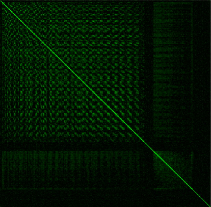
We notice a couple of things here. First, as noted before, there is a diagonal line traversing the matrix. Secondly, it is symmetrical on either side of the line since $Cor(X,Y) = Cor(Y,X)$. We also see some common frequency domain behavior in this picture. We know sinusoidal components in the input signal are probably affecting multiple frequency bins. Because of this, bins close together tend to correlate similarly with the same frequency bins. This can be seen as a checkered pattern in the matrix. Particularly quiet sections of the spectrum are also shown in the matrix. These are the dark sections. Regions that are most likely filled with discrete spectral noise don’t correlate well with anything intentional, and thus aren’t bright. Perhaps the most important thing to take away from this picture is the width of the diagonal line. We expect this to be the brightest part of the picture, which indeed it is. For each frequency at a given point on the Y-axis, the width of the horizontal line at that point tells us how strongly the amplitude difference envelope of that frequency correlates with that of the frequencies around it. Consequently this give us a sense of how likely those bins are as targets for sinusoidal movement from a given location. Furthermore, we see that the width of the line appears to get a bit wider the further in the spectrum we go. This also makes sense given that, in musical signals, higher frequency components in the spectrum travel a further frequency distance than lower frequency components. 

So how good of a representation is this matrix of signal structure? For comparison, let’s see what matrix is drawn for a signal with no structure.

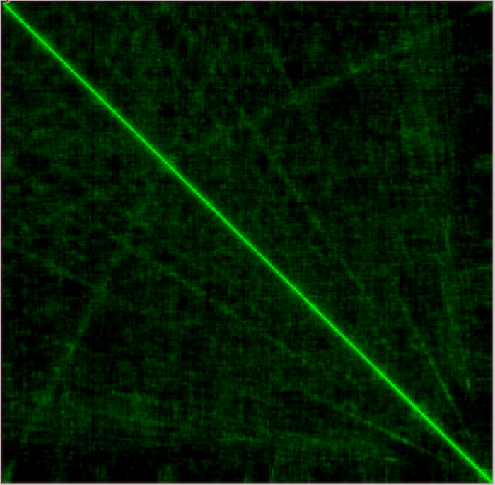
As we can see, there is far less apparent structure in the correlation matrix. The checkered behavior as well as the dark regions we saw earlier don’t show up in this picture. Furthermore, since this input doesn't really have a sinusoidal structure like a musical one does, what the FFT perceives as sinusoidal components are affecting many frequency bins at once. This is displayed as a very wide diagonal line throughout the spectrum. So it seems like this correlation matrix is an accurate representation of how structured its input signal is.

Conclusion 

We have given the motivation to why a statistical investigation into the phase vocoder is warranted, some practical considerations and methods for going about these calculations, and shown some promising first results when we assume the phase vocoder is a Markov chain and carry out the subsequent ideas. Looking forward to next post, we will investigate how we can use this correlation matrix data to help create a more accurate transition matrix, how these pictures and transition matrices are represented in phase vocoder improvements, and what they suggest for future algorithms. 

Read the original post here where we approach this idea using Max/MSP. 

Code

MATLAB

Max/MSP

References

[1] https://en.wikipedia.org/wiki/Markov_property

[2]

pdf download

Sign in