


Reduced-Delay IIR Filters
This blog gives the results of a preliminary investigation of reduced-delay (reduced group delay) IIR filters based on my understanding of the concepts presented in a recent interesting blog by Steve Maslen [1].
Development of a Reduced-Delay 2nd-Order IIR Filter
Maslen's development of a reduced-delay 2nd-order IIR filter begins with a traditional prototype filter, HTrad, shown in Figure 1(a). The first modification to the prototype filter is to extract the b0 feedforward coefficient path from the filter's delay line as shown in the HMod filter presented in Figure 1(b).
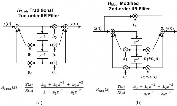
Figure 1. Equivalent 2nd-order IIR filters: (a) prototype traditional filter, HTrad;
(b) modified filter, HMod.
As shown in Appendix A, the two filters' HTrad(z) and HMod(z) z-domain transfer functions given in Figure 1 are identical. The final step in Reference [1]'s modifications is to shift HMod's two feedforward coefficients upward in the delay line to produce the desired reduced-delay 2nd-order IIR filter, HRed‑Del, shown in Figure 2.
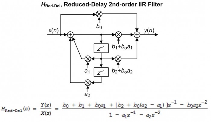
Figure 2. Reduced-delay 2nd-order IIR filter.
The derivation of the HRed‑Del(z) transfer function in Figure 2 is given in Appendix B.
Performance of a Reduced-Delay 2nd-Order IIR Filter
Reference [1] states that, relative to the prototype Figure 1(a) filter, the Figure 2 filter will have a group delay reduced by one sample time. As it turns out, the Figure 2 filter does indeed have a reduced passband group delay, but the interesting thing is that the amount of group delay reduction depends on the nature of the original prototype filter.
We show this behavior in Figure 3 for four traditional prototype lowpass 2nd-order filters; the so-called Butterworth, Elliptic, Chebyshev Type-1, and Chebyshev Type-2 filters.
The filters, whose cutoff frequencies are 1/8th of their sample rate, were designed using one of the following MATLAB commands:
[b,a] = butter(2, 0.25);
[b,a] = ellip(2, 2, 30, .25);
[b,a] = cheby1(2, .5, .25);
[b,a] = cheby2(2, 30, .25);
The first column of Figure 3 shows the z-plane pole/zero locations for the prototype traditional IIR filters, while the second column shows the z-plane pole/zero locations for the Figure 2 reduced-delay filters.
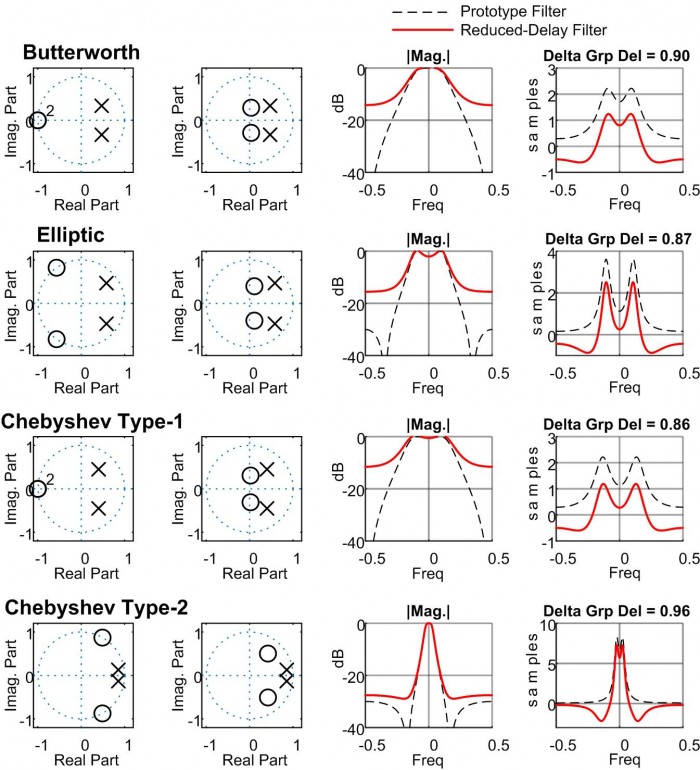
Figure 3. 2nd-order lowpass prototype filter and reduced-delay filter performance. First column is the z-plane of the prototype filter, the second column is the z-plane of the reduced-delay filter.
Because the prototype –to- reduced-delay filter conversion process modifies a prototype filter’s feedforward coefficients, notice how that process shifted the locations of the z-plane zeros for the reduced-delay filters and this affects their stopband attenuation.
In the third column of Figure 3 the dashed and solid curves show the frequency magnitude responses of the lowpass prototype traditional and Figure 2 reduced-delay filters respectively. Notice the reduced stopband attenuation of the reduced-delay filters’ solid curves in the third column.
In the forth column of Figure 3 the dashed and solid curves show the group delay plots of the lowpass prototype traditional and Figure 2 reduced-delay filters respectively. The ‘Delta Grp Del’ label above the fourth column’s plots give the group delay reduction of the reduced-delay filters at zero Hz (measured in samples).
What We Should Learn From Figure 3
Regarding Reference [1]’s IIR filter group delay reduction process producing the Figure 2 filter, the main points of this blog are:
• The amount of group delay reduction in the passband of the Figure 2 reduced-delay filters is just less than one sample.
• Relative to the original prototype IIR filters, the stopband attenuation of the reduced-delay filters is significantly degraded.
• The amount of group delay reduction and the stopband attenuation of the reduced-delay filters depends on the design method of the original IIR filter being converted.
If this reduced-delay filter topic interests you, the PDF file associated with this blog presents the performance of 1st-, 3rd-, and 4th-order reduced-delay IIR lowpass filters.
References
[1] Maslen, Steve, "Part 11. Using -ve Latency DSP to Cancel Unwanted Delays in Sampled-Data Filters/Controllers", Website: dsprelated.com, https://www.dsprelated.com/showarticle/1280.php
Appendix A: Proof of HMod(z) = HTrad(z)
Proving the equivalence of Figure 1's HTrad(z) and HMod(z) transfer functions begins by expressing HMod(z) as:

Putting the two terms in Eq. (A-1) over a common denominator yields:

Collecting the factors of z in Eq. (A-2) gives us:

Canceling the appropriate positive and negative terms in Eq. (A-3) gives us HMod(z)'s transfer function that is equal to the traditional IIR filter's HTrad(z) given as:

Appendix B: Derivation of HRed-Del(z) Transfer Function
The derivation of the Figure 2’s HRed-Del(z) transfer function proceeds as follows:

Putting the two terms in Eq. (B-1) over a common denominator yields:
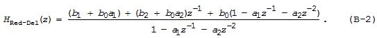
Collecting the factors of z in Eq. (B-2) gives us the desired 2nd-order HRed-Del(z) z-domain transfer function:

- Comments
- Write a Comment Select to add a comment

Thanks Rick. I guess there's no free lunch.

Hi Neil. You're right.
The purpose of my study was to merely find out how the ‘delay reduction modification’ affects the performance of simple IIR filters. The modification does reduce a filter’s group delay but the price you pay in terms of degraded attenuation is high.

Hi Rick,
Are you referring to degradation of modified filter. This modified section is not relevant. Its top branch needs be considered as part of it hence it is equivalent to prototype filter. Am I right?
Of course the purpose is not to make costly modification for a worse filter but that same prototype performance is to be expected yet less delay in lower branch processing
Thanks
Kaz
Hi Kaz.
Your "Comment" has made me insert a few adjectives in the text of my blog to make it super clear that the black curves in the 3rd & 4th columns of Figure 3 give the freq-domain performance of the Figure 1(a) prototype traditional 2nd-order IIR filters. And the red curves in the 3rd & 4th columns of
Figure 3 give the performance of the Figure 2 'reduced-delay' 2nd-order IIR filters.
[There's no need to discuss the performance of the Figure 1(b) "modified" filter because that filter is equivalent to the Figure 1(a) filter.]
I don't understand what you 2nd paragraph is saying. The Figure 2 'reduced-delay' filter, and the other-order 'reduced-delay' filters described in the PDF file, are dual-path (two-branch parallel) filters. And my analysis of those filters' performances are for the dual-path filters. I did NOT analyze the behavior of any single branch of any dual-path filter. I hope what I wrote makes sense.
Hi Rick,
I assumed the filter functionality is not degraded. I am repeating here the time domain direct analysis using random input, the error is of the order 10^-15 for floating point case and with my arbitrary coeffs:
%%%%%%%%%%%%%%%%%%%%%%%%%%%%%%%%%%%%%%%%%
x = randn(1,1024);
b0 = 0.1; b1 = .376; b2 = -.71;
a0 = 1; a1 = -.7; a2 = .72;
y1 = filter([b0,b1,b2],[a0,a1,a2],x);
y2 = filter([b1-b0*a1,b2-b0*a2,0],[a0,a1,a2],x);
y2 = x*b0 + [0 y2(1:end-1)];
plot(y1,'.-');hold;
plot(y2,'g.--');
figure;(plot(y1-y2));
%%%%%%%%%%%%%%%%%%%%%%%%%%%%%%%%%%%%%%%%
so I can see discrepancy between my analysis and yours. Not sure why?
Hi kaz. I think the discrepancy is your:
y2 = x*b0 + [0 y2(1:end-1)];
command. Instead of a noise input try using a unit impulse input using the following:
[Numer, Denom] = butter(2, 0.25); % Lowpass:
b0 = Numer(1); b1 = Numer(2); b2 = Numer(3);
a1 = -Denom(2); a2 = -Denom(3);
x = 1; x(40) = 0;
a0 = 1; a1 = -a1; a2 = -a2;
y1 = filter([b0,b1,b2],[a0,a1,a2],x);
y2 = filter([b1-b0*a1,b2-b0*a2,0],[a0,a1,a2],x);
y2(1) = b0 + y2(1);
Notice that I replaced your
y2 = x*b0 + [0 y2(1:end-1)];
command with the following command:
y2(1) = b0 + y2(1);
Now that you have a 'y2' impulse response for a lowpass filter, you can compute the FFT's magnitude of that impulse response to see the freq magnitude response of a 'reduced-delay' lowpass filter. (You can also compute the impulse response of the original 'b' and 'a' coefficients and obtain the original lowpass filter's freq magnitude response.
By the way, I see that you used Maslen's transfer function to compute your y2 sequence instead of using the transfer function in my Figure 2. (My Figure 2 adds the feedback values to the 'x' input where Maslen's block diagram subtracts the feedback values from the 'x' input.)
Am I missing something? These "equivalent" filters look pretty dismal! for Butterworth filter, over half of the (logrithmic) attenuation is lost! For the elliptic and Chebychev filters, less is lost, but these filters are used when a lot of attenuation is required, which you lose when applying the modification.
One other unrelated question: I never heard of a first order elliptic or Chebyshev filter. In the analog domain, these filter (Butterworth/Chebyshev/elliptic) types differ in the shape of the pole distribution (on circle for Butterworth filter, etc.) and the presence/absence of zeros. How can one change the shape of a filter with only 1 (real) pole? The only degree of freedom is the magnitude of the feedback term, and the overall scaling term (affects overall gain only, not shape). For the unmodified 1st order filters, the Chebyshev filter has a response that is less sharp then the Butterworth! All of the 1st order filters have their output "destroyed" by the modification!
Hello Brian. No, you did not "miss" anything. It sure looks like those 'reduced-delay' filters have rather limited utility.
Did you read the Reference [1] blog when it was first posted by Steve Maslen? If so, didn't his blog pique your interest in learning more about his proposed 'reduced-delay filter modification' process?

Hi Folks,
Nice to to see some spin-off analysis and discussion.
Just to clarify a few matters.
1) The purpose of the arrangement as I described it is not at this stage to make improvements to the characteristics of digital filters. e.g. to take a well-known abstract IIR filter response and somehow make it have some beneficial behavior.
2) The purpose so far has been to enable my desired digital filter characteristics to be realizable in a circuit such that I have input-output signals that for practical purposes, precisely match those that might have been obtained from an analogue circuit. Normally this is not possible in a sampled-data system due to the delays from the ADC acquisition time, Computation time and DAC reconstruction effects.
The basic arrangement described allows the desired characteristic to actually be achieved whereas a single path ADC --> Digital Filter --> DAC can never produce the required result.
Its true there are no free lunches, but if you absolutely must have a practical time-faithful transfer function of the types documented, then the addition of a simple gain and a bit of coefficient manipulation is not much effort if necessity calls.
Steve
Hi Steve. I can certainly believe that your 'reduced-delay modification' process could prove to be useful in some specific signal processing application.
For the sake of clarity, all these modified filter responses can be implemented using a traditional topology as well. I believe the takeaway here is that moving the holes and poles towards zero will reduce the group delay. Focusing on group delay is something I believe is a worth while endeavor. However, I have a hard time seeing the benefit in trying to cheat a single sample of group delay by relocating holes. I agree with Mr Lyons that there is most likely some application for which this could prove useful, but I can’t think of one immediately.
Hi dszabo. There may be more than one conversation going on here so I'm not sure if your comments were only for Rick. I believe that Rick has been looking at the possibilities for improving traditional filter responses. My area of interest is in fast closed-loop control applications. Unwanted delays really do matter in this area and make the difference between a solution that works and a solution that does not. For these applications, the provision of an extra degree of freedom that removes unwanted delays is an engineering innovation rather than a cheat.
I apologize for my poor choice of terminology. I did not mean cheat in the sense of cheating. I genuinely believe that there is not cheating in signal processing, and certainly do not believe that proposing an alternative filter topology is cheating. I was intending to use the term in the sense of “cheating” your idle rpm on your engine to keep it from stalling, or adding an extension to a ratchet wrench to get some extra torque. Thank you for taking the time to contribute to this site, as it is my favorite forum for the topic. I’ve very much enjoyed your blog posts on closed loop control loops
Hi dszabo, No worries (as the Australians say:-) and thank you for the kind comments. I may write a bit more to show the impact of a 1 sample delay on a closed-loop response and the detailed design to overcome the problem.
Hi dszabo. Your first sentence intrigued me. Can you describe how you would use "traditional topology" to implement a 'modified dual-path' filter?
If we define the first filter topology as traditional, in that it is well documented, then we know from the transfer function that any discrete time biquad filter can be implemented. We also know that the transfer function is equal to the product of the numerator (holes) and the denominator (poles). As you have shown with your analysis, the modified dual path implementation only affects the locations of the holes, because the denominator is unchanged. Therefor, we calculate the coefficients of the modified filter transfer function and plug them into the traditional one and get the same result. Equivalently, one could calculate the new hole locations and use those to calculate the new filter coefficients.
What I believe is interesting is that it can be observed (I’ve done this emperically, but have not proved it analytically) that the group delay for the numerator of a second order filter is two samples at maximum (I.e z^-2) and zero at minimum (I.e 1). In many filter strategies such as the ones you used in your example, the zeroes are located on the unit circle, which corresponds to a maximum group delay of 1 (again, I’ve only checked this empirically). If one were serious about reducing the group delay, one would place the zeroes at zero, setting the numerator to one, giving the lowest group delay for the numerator. This would also reduce the attenuation of the filter, severely impacting filter performance. In fact, I would speculate that many in many applications, an IIR filter’s group delay is primarily a factor of the poles, which the modified topology does not address.
And come one, who is really fighting over, best case, one sample of group delay?
Hi dszabo. You wrote:
"Therefor, we calculate the
coefficients of the modified filter transfer function and plug them into
the traditional one and get the same result."
Ah, OK, now I understand what you mean. The result of your above statement is the H_Red-Del(z) transfer function that I presented in my Figure 2.
Someone with a low sample rate possibly...
Very interesting article,
It seems the benefit of reducing the lag by at most a sample needs to be weighed with the reduction of attenuation in the stopband.
I believe the group delay can be reduced a little bit more with the realization of weighted filter('s) in parallel with the one proposed above, of course sacrificing some amount of further reduction in the stopband. This is done by creating an 'equi-ripple' group delay for the passband frequencies instead of a single peak group delay near the cutoff. This is achieved by tuning a complementary weight on an emva and a reduced delay butterworth filter in parallel that each have relatively the same max group delay.
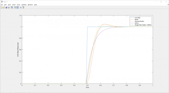
The unit step seems to have optimal rise time, settling time. I apologize in advance if this is off topic or I have made an error somewhere, just thought it was noteworthy.
Matlab Code:
clear all, close all, clc

Nf = 2000;
Fs = 100;
t = 0:1/Fs:1;
x = (t >= 0.5);

% Butter filter
Num1 = [ 0.020083365564211235615443840174521, 0.040166731128422471230887680349042, 0.020083365564211235615443840174521];
Den1 = [ 1.0, -1.561018075800718163392843962356, 0.6413515380575630642212558996107];
y1 = filter(Num1, Den1, x);
[H1, wn] = freqz(Num1, Den1, 'half', Nf);
gd1 = grpdelay(Num1, Den1, Nf);

% Reduced Delay Butter filter
Num2 = [ 0.091600593361281137938512131313473, -0.024147628498415365377871566465728, 0.012880497393979173370581747803953];
Den2 = [ 1.0, -1.561018075800718163392843962356, 0.6413515380575630642212558996107];
y2 = filter(Num2, Den2, x);
[H2, ~] = freqz(Num2, Den2, 'half', Nf);
gd2 = grpdelay(Num2, Den2, Nf);

% EMVA IIR
Num3 = [0.18542572959112146868676518352004];
Den3 = [ 1.0, -0.81457427040887853131323481647996];
y3 = filter(Num3, Den3, x);
[H3, ~] = freqz(Num3, Den3, 'half', Nf);
gd3 = grpdelay(Num3, Den3, Nf);

% Further Reduced Delay Butter Filter
Num4 = [ 0.12443939104172524467983862450637, -0.16550454521665269869146186465514, 0.062780924173166358093212124913407, -0.0068198791486826304888979599638787];
Den4 = [1.0, -2.3755923462095966947060787788359, 1.9129166982480043657233181875199, -0.52242846118885155615174653576105];
y4 = filter(Num4, Den4, x);
[H4, ~] = freqz(Num4, Den4, 'half', Nf);
gd4 = grpdelay(Num4, Den4, Nf);

f = wn*Fs / (2*pi);
figure(1);
plot(t, [x', y1', y2', y3', y4']); ylabel('Unit Step Response'); xlabel('time');
legend('Unit Step', 'Butter', 'Reduced Butter', 'EMVA', 'Weight Red. Butter + EMVA')

figure(2);
subplot(121);
plot(f, [abs(H1), abs(H2), abs(H3), abs(H4)]); ylabel('Magnitude'); xlabel('frequency (Hz)');
legend('Butter', 'Reduced Butter', 'EMVA', 'Weight Red. Butter + EMVA')

subplot(122);
plot(f, [gd1, gd2, gd3, gd4]); ylabel('Group Delay (samples)'); xlabel('frequency (Hz)');
legend('Butter', 'Reduced Butter', 'EMVA', 'Weight Red. Butter + EMVA')
To post reply to a comment, click on the 'reply' button attached to each comment. To post a new comment (not a reply to a comment) check out the 'Write a Comment' tab at the top of the comments.
Please login (on the right) if you already have an account on this platform.
Otherwise, please use this form to register (free) an join one of the largest online community for Electrical/Embedded/DSP/FPGA/ML engineers:


