


The Zeroing Sine Family of Window Functions
Introduction
This is an article to hopefully give a better understanding of the Discrete Fourier Transform (DFT) by introducing a class of well behaved window functions that the author believes to be previously unrecognized. The definition and some characteristics are displayed. The heavy math will come in later articles. This is an introduction to the family, and a very special member of it.
This is one of my longer articles. The bulk of the material is in the front half. The back half is mostly example numbers and sample code empty of much explanatory material.
The Work Horse That Started it All
A window function acts like a filter on the DFT values as if they were a signal. The VonHann is one of the simplest, yet most powerful ones. It is equivalent to doing a 0.5( 1, -2, 1 ) filter on the DFT. This is the same as the second difference calculation. What it does is wipe out all "best fit lines" within each three bin set.
A similar "filter" arises naturally out of my frequency formula derivations. It doesn't wipe out the best fit line, but nearly so.
Let $ r = e^{-i\frac{2\pi}{N}} $. Then the definition of the vector is: $$ (-1, 1+r,-r) = r^{1/2} ( -r^{-1/2}, r^{-1/2} +r^{1/2}, -r^{1/2} ) \tag {1} $$ In the formulas, the vector can be multiplied by any scalar, as it appears linearly in the numerator and denominator of the formulas. $$ \begin{aligned} ( -r^{-1/2}, r^{-1/2} +r^{1/2}, -r^{1/2} ) &= ( e^{i\frac{\pi}{N}}, e^{i\frac{\pi}{N}} + e^{-i\frac{\pi}{N}}, e^{-i\frac{\pi}{N}} )\\ &= ( e^{i\frac{\pi}{N}}, 2 \cos \left( \frac{\pi}{N} \right), e^{-i\frac{\pi}{N}} ) \end{aligned} \tag {2} $$ The filter guys might recognize the same rescaled (acting as a shift) vector as: $$ z ( 1, -2 z^{-1} \cos \left( \omega \right), z^{-2} ) \tag {3} $$ When dotted with $(1,1,1)$, aka "DC" this vector becomes: $$ \begin{aligned} ( 1, -2 z^{-1} \cos \left( \omega \right), z^{-2} ) \cdot(1,1,1) &= 1 -2 z^{-1} \cos \left( \omega \right) + z^{-2} \\ &= (1)^2 + (z^{-1})^2 - 2 (1)(z^{-1}) \cos \left( \omega \right) \end{aligned} \tag {4} $$ The last equation is the Law of Cosines, so you know it isn't a contrived fluke.
The corresponding window function is: $$ w[n] = \sin \left( \frac{n}{N}\pi \right) \sin \left( \frac{n+1}{N}\pi \right) \tag {5} $$ What is notable is that it zeros out the last sample as well as the first. This can easily be confirmed by plugging in $n=0$ and $n=N-1$ into the equation. One factor covers one end, the other the other.
The question was posted in the forum on this site on whether anybody recognized this window function, or thought it was anything special. Only one expert stepped forward and confirmed it was unknown to them. This was not unexpected and similar to my experience with presenting other new ideas. Since no one recognized the vector that the rest of this article is based on, it is likely it is novel too.
The Original Formulation of the Family
Expanding on this observation is straightforward. A family of window functions can be built up by including one more sine term for each level. Originally, they were stacked so that the points on the ends were zeroed towards the middle. $$ \begin{matrix} 0 & 1 & 1 \\ 1 & \sin\left( \frac{n}{N}\pi \right) & \\ 2 & \sin\left( \frac{n}{N}\pi \right) \sin\left( \frac{n+1}{N}\pi \right) & \\ 3 & \sin\left( \frac{n-1}{N}\pi \right) \sin\left( \frac{n}{N}\pi \right) \sin\left( \frac{n+1}{N}\pi \right) & \\ 4 & \sin\left( \frac{n-1}{N}\pi \right) \sin\left( \frac{n}{N}\pi \right) \sin\left( \frac{n+1}{N}\pi \right) \sin\left( \frac{n+2}{N}\pi \right) & \\ \end{matrix} \tag {6} $$ This leads to the zeroing pattern shown on an eight sample frame:
   n =      01234567
        0 T|TTTTTTTT|T
        1 .|0...T...|0
   L =  2 0|0..tt..0|0
        3 0|00..T..0|0
        4 0|00.tt.00|0
The T's stand for the "Top" value. The symbol even looks made for the part. A dot is a non zeroed value. The vertical characters demarcate the frame. The even/odd pattern is obvious.
Left Fill Formulation
From a math point of view, filling zeroes from the left is equivalent and simpler to formulate. The distinction is one of referencing, not behavior. Here is the corresponding zeroing pattern:
    0 T|TTTTTTTT|T
    1 .|0...T...|0
    2 0|00..tt..|0
    3 0|000..T..|0
    4 0|0000.tt.|0
So, I worked all the math that way.
An Endian Transformation
After working through it for a while, rather than have the zeros left fill the frame, it makes more sense to have them fill from the right.
Sorry for any whiplash. Oh, you didn't feel it? I sure did. The symmetry is quite clear. Reverse the indexing direction and you get the equivalent definition so they have to be forward and backward symmetric.
The right zero padding family is: $$ \begin{aligned} W_0 &= 1 \\ W_1 &= \sin \left(( n + 1 ) \frac{\pi}{N} \right) \\ W_2 &= \sin \left(( n + 1 ) \frac{\pi}{N} \right) \sin \left(( n + 2 ) \frac{\pi}{N} \right) \\ W_3 &= \sin \left(( n + 1 ) \frac{\pi}{N} \right) \sin \left(( n + 2 ) \frac{\pi}{N} \right) \sin \left(( n + 3 ) \frac{\pi}{N} \right) \\ W_4 &= \sin \left(( n + 1 ) \frac{\pi}{N} \right) \sin \left(( n + 2 ) \frac{\pi}{N} \right) \sin \left(( n + 3 ) \frac{\pi}{N} \right) \sin \left(( n + 4 ) \frac{\pi}{N} \right) \\ \end{aligned} \tag {7} $$ It's easy to see that the first member zeroes out the $N-1$ sample. The next does that and $N-2$, and so on. The subscript to the window function indicates how many samples are zeroed out.
Here is the corresponding zeroing pattern for a frame size of nine:
    0 T|TTTTTTTTT|T
    1 .|...tt...0|0
    2 0|...T...00|0
    3 0|..tt..000|0
    4 0|..T..0000|0
For purposes of analysis, the future can be zeroed out for a little while so you don't have to wait for it to happen. Also, the zeroing allows the calculation of the DFT to be reduced if coded properly. The non-zero stretch is the stance on the signal when this is used as a window function. The zero padding is how zero padding should be done.
In other words, the placement of the zero stretch and non-zero stretch is simply a matter of referencing. The true behavioral reference is the peak of the curve.
The Simplified Formulation
The window functions can also be more simply represented by using a variable substitution for the discrete angles. $$ \begin{aligned} \psi &=\frac{n}{N}\pi \\ \chi &=\frac{1}{N}\pi = \frac{1}{2} \beta_1 = \frac{1}{2} \left( \frac{2\pi}{N} \right) \\ \end{aligned} \tag {8} $$ The $\beta_1$ is my consistent representation of 1/Nth of a circle. Note that $\chi$ is half of that. The sine function only goes half a cycle in the frame since $\psi=n\chi$ only takes half the root angle (a semi-root) step each sample. This means it can only zero out one sample within the DFT frame no matter how it is shifted.
Using the variable substitutions also loosens the tie to their presumed values and let's the equations be viewed on a continuous basis. Even though we are dealing with a specific case, we can think of it in a general framework. $$ \begin{aligned} W_0 &= 1 \\ W_1 &= \sin(\psi + \chi ) \\ W_2 &= \sin(\psi + \chi ) \sin(\psi + 2 \chi ) \\ W_3 &= \sin(\psi + \chi ) \sin(\psi + 2 \chi ) \sin(\psi + 3 \chi ) \\ W_4 &= \sin(\psi + \chi ) \sin(\psi + 2 \chi ) \sin(\psi + 3 \chi ) \sin(\psi + 4 \chi ) \\ W_5 &= \sin(\psi + \chi ) \sin(\psi + 2 \chi ) \sin(\psi + 3 \chi ) \sin(\psi + 4 \chi ) \sin(\psi + 5 \chi )\\ \end{aligned} \tag {9} $$ The window functions are a product of shifted Sines. They are very factorial like in their definition. $$ W_L = \prod_{l=1}^{L} \sin(\psi + l \cdot \chi ) = \prod_{l=1}^{L} \sin \left( \frac{n+l}{N}\pi \right) \tag {10} $$
The Recursive Formulation
The window family members can be defined via their predecessors, and values evaluated this way in code. $$ \begin{aligned} W_0 &= 1 \\ W_1 &= W_0 \sin(\psi + \chi ) \\ W_2 &= W_1 \sin(\psi + 2 \chi ) \\ W_3 &= W_2 \sin(\psi + 3 \chi ) \\ W_4 &= W_3 \sin(\psi + 4 \chi ) \\ W_5 &= W_4 \sin(\psi + 5 \chi )\\ \end{aligned} \tag {11} $$ A simple recursive definition is: $$ \begin{aligned} W_L &= W_{L-1} \sin(\psi + L \chi ) \\ \end{aligned} \tag {12} $$ Plainly, each next member has one more root. When aligned with samples they will be zeroed out. Ultimately a sample aligned $W_N$ will zero every sample in a $N$ sized frame, yet will not be the zero function. By symmetry each sample interval will be identical.
The definition of $W_0 = 1$ is one of convenience. Notice that is acts like a coefficient for the rest of the calculation. The same superstructure can be built on top of any $W_0$, without having to be recalculated.
The recursive definiton can be evaluated in either row major or column major order. Here is a code snippet from the program that produces the tables below:
#---- Set parameters

        N = 9
        L = 7

        theChi = np.pi / N

#---- Allocate the Family

        theFamily = []

        for l in range( L ):
          theFamily.append( np.zeros( N ) )

#---- Build the Zeroing Sine Family

        for n in range( N ):

          theFamily[0][n] = 1.0

          for l in range( 1, L ):
            theFamily[l][n] = theFamily[l-1][n] * np.sin( (n+l)*theChi )
There is a slightly better code snippet at the end of Appendix II and an even better one in Appendix V.
DFT Indexing and Framing
These DFTs are portrayed with the conventional $0$ to $N-1$ indexing. From a theoretical viewpoint, it is much simpler to consider only odd sized DFTs and to center the zero sample in the signal and the DC bin in the spectrum. However, it is well known that FFT implementations are most efficient having frames with power of two sizes and most are zero based. Just as the location of the zeroes can be slid around without behavioral consequence, so too can the choice of reference frames for the DFT be made.
The Fourier Formulation
There are binomials in the definitions, and they are multiplied together in patterns. This means the Pascal's triangle pattern is going to come into play. This is illustrated in Appendix III to generate the Fourier Series coefficients for the window function family.
As a result, the window functions can be defined by the sum of sine and cosines of the half fundamental for the frame and its harmonics.
The number of terms rises quickly for each family member. An algortihmic solution is fairly straight forward and was used to generate the demonstration grid. The member of the family can then be defined as a set of three member integer tuples "(coeffient, n step, 1 step)" and expanded using a double-wide semi-roots trig lookup table.
This allows for alternative formulas without powers, but their complexity makes this impractical. They are essential for the mathiness of it all.
Values in a Small Frame
Here are some values on an $N=9$ frame. Spinning a signal up by Nyquist before the DFT has the effect of shifting the bin values so the original DC ends up at Nyquist. For these displays, centering the DC is desirable.
  L =   0        1        2        3        4        5        6

Window Function

  0  1.0000   0.3420   0.2198   0.1904   0.1875   0.1847   0.1599
  1  1.0000   0.6428   0.5567   0.5482   0.5399   0.4676   0.3005
  2  1.0000   0.8660   0.8529   0.8399   0.7274   0.4676   0.1599
  3  1.0000   0.9848   0.9698   0.8399   0.5399   0.1847   0.0000
  4  1.0000   0.9848   0.8529   0.5482   0.1875   0.0000  -0.0000
  5  1.0000   0.8660   0.5567   0.1904   0.0000  -0.0000   0.0000
  6  1.0000   0.6428   0.2198   0.0000  -0.0000   0.0000  -0.0000
  7  1.0000   0.3420   0.0000  -0.0000   0.0000  -0.0000   0.0000
  8  1.0000   0.0000  -0.0000   0.0000  -0.0000   0.0000  -0.0000

DFT of Window spun up by Nyquist

  0  1.0000   0.0000   0.0622   0.0000   0.0226   0.0000   0.0193
  1  1.0642   0.0000   0.0764   0.0000   0.0346   0.0000   0.0555
  2  1.3054   0.0000   0.1527   0.0000   0.1875   0.2813   0.2450
  3  2.0000   0.0000   0.8264   1.1250   1.0798   0.8098   0.4605
  4  5.7588   4.5000   3.6454   2.8486   2.0293   1.2407   0.6011
  5  5.7588   4.5000   3.6454   2.8486   2.0293   1.2407   0.6011
  6  2.0000   0.0000   0.8264   1.1250   1.0798   0.8098   0.4605
  7  1.3054   0.0000   0.1527   0.0000   0.1875   0.2813   0.2450
  8  1.0642   0.0000   0.0764   0.0000   0.0346   0.0000   0.0555

DFT of Window spun up by Nyquist and a half

  0  0.0000   0.1820   0.0000   0.0352   0.0000   0.0223   0.0000
  1  0.0000   0.1820   0.0000   0.0352   0.0000   0.0223   0.0000
  2  0.0000   0.2376   0.0000   0.0661   0.0000   0.0983   0.1406
  3  0.0000   0.4465   0.0000   0.3808   0.5625   0.5317   0.3561
  4  0.0000   1.9696   2.2500   2.0606   1.6197   1.0634   0.5455
  5  9.0000   5.6713   4.2286   3.1570   2.1822   1.3044   0.6204
  6  0.0000   1.9696   2.2500   2.0606   1.6197   1.0634   0.5455
  7  0.0000   0.4465   0.0000   0.3808   0.5625   0.5317   0.3561
  8  0.0000   0.2376   0.0000   0.0661   0.0000   0.0983   0.1406
The first thing to notice is that the window functions do indeed zero out the first some many samples according to the level.
The second two blocks show the "leakage" remediation capability. The first column is the no window, or frame rectangular window, window function, the second column is a half sine. These are known window functions. The third column is the work horse, a VonHann like window. The rest are "new". Notice that the DFTs in the last column have almost the same profile, making the appearance in the DFT very bin independent.
The even/odd pattern typical in DFT comes into play as well. Since the odd members of the family are oriented on the half bin, the DFT of the half twist is very concentrated in the spectrum. Likewise, the even members are the most concentrated on the whole bin and most leakage on the half twist. This distinction goes away as the levels climb.
Values in a Large Frame
Here are the first hundred members of the family on a frame of 630 samples in black. The red are the rescaled DFT values for the last ten members by steps of ten.
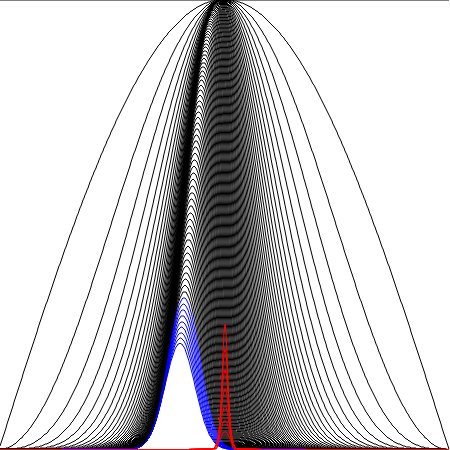
Most prominently, the window functions are approaching a Gaussian shape, and at some point will overshoot that. They are not true Gaussians. Likewise, the DFT values are also approaching a Gaussian shape.
When N is large and L is small, the window functions should behave very much like their Raised Sine counter parts. When L gets large compared to N, things get more interesting.
The Shrinking Window
For every level up in the family, the next member zeroes out one more sample. This shrinks the size of the samples used, but not the size of the DFT frame. It is as if there is a shorter sampling frame ($N-L$) followed by zero padding ($L$).
The Stance on the DFT
The zeroth member, the unit rectangle window that fits the frame, has a bin stance of one bin. Every additional member of the Zeroing Sine windows takes up one more bin width in the stance. For even N, the bin stance is on the half bins, and for odd N it is on the whole bins. The size of the bin stance is then $1+L$, leaving $N-(L+1)=(N-1) - L$ zero valued bins.
For odd sized bin stances, the spectrum is centered on DC. For even sized bin stances it shifts half a bin. This explains the stances being revealed in the even/odd pattern shown for the N=9 case above. The stances can be seen by summing across the horizontal columns in Appendix I. They follow the Pascal's triangle binomial distribution pattern, but not quite the value pattern.
The Very Special Family Member
So, as the number $L$ increases, in the signal domain there is a shrinking window of $N-L$ non-zeroed samples. Meanwhile in the spectrum, aka frequency domain, there is a growing bin stance of $L+1$ bins. They both look like Gaussians.
Could it be that if we line them up and that they might be multiples of each other? Finding the $L$ value for which the zero profile in the signal domain matches the spectrum is easy: $$ \begin{aligned} N - L &= L + 1 \\ L &= ( N - 1 ) / 2 \end{aligned} \tag {13} $$ $L$ will only be an integer with odd N. So, the peaks will only align on the non-zeroed/zeroed profiles for odd DFT frame sizes. Numerically, this is confirmed.
The $L=(N-1)/2$ member of odd $N$ families turns out (numerically, working on a proof) to be an exact base Discrete Hermite-Gaussian DFT Eigenvector. This was hoped for, and greatly satisfying when confirmed.
The Crazy Uncle Family Member
The even $N$ case presented quite a challenge. The technique that works was tried early and failed, so failure of the test, not the concept. So a lot of trails in the new territory were explored.
The fix is simple. Find the family member that takes the first half of the frame. Then add it to itself one spot over. This shifts the center half a bin and makes the number of non-zero bins match the DFT stance. The proof of why it works isn't that hard using the definition.
Likewise, if one window function can subtracted from a shifted version of itself (the difference operator), or any kind of combination, particularly binomial combinations, will yield similar curves. The rules still need to be worked out. For instance, a "tt" top slid and subtracted will yield a zero crossing, a "T" top won't.
It would be reasonable to expect to find the higher order Discrete Hermite-Gaussian eigenvectors among this extended set in a regular pattern. The reader is encouraged to find the pattern first by starting with the source code listing in Appendix V and making appropriate modifications, as I will be doing at some point. The mathematician reader is also encouraged to work out the same using the definition (10), as I will be doing at some point. [If you accomplish either before I do, please make reference in the comments.]
There will be another article (or two) on the Eigenvectors found. This article shows the path to the doorway of a whole set of new patterns.
Ideal for a Spectrogram
For a 1024 sample DFT, a window size of about 140 samples will cover a swath within the range of CD quality. That means a 140 sample range can be nestled up to the leading edge of real time data, with a latency of 70 samples, yet have 1024 sample resolution behind it. Sort of like having a 7X magnifying glass in terms of frequency resolution. This window is like the ideal corrective lens for the DFT so that continuous changes in the underlying parameters are undistorted in the spectrum.
Never is there any uncertainty involved in the smearing. The same pure tone will be fond in the place every time, at the center of the distribution. If you have a wavering/noisy tone, the best fit will be at the center and you smear will be wider. Since the first is known definitionally, the difference in smear widths can be used to measure the off-pure-tone-ness (distortion?).
For a spectrogram, on a log scale, standalone modes will be approximate parabolas (exact at center). This lead to simple and accurate interpolation for display purposes freeing the need to be bin aware for selection criteria.
Multiple Tone Decomposition
Every pure tone, no matter what the bin alignment, gets smeared into the same eigenvector Gaussian shape in the magnitude profile of the spectrum. It is the ideal manifestation of the DFT "acting like a FT", only smeared. The smearing should not be interpreted as "uncertainty", it is simply the mechanism to put all frequencies, no matter what their frequency fraction value is, on a non-discriminatory continuous scale. The width of the smear is well defined for a tone, so any distortion and noise will show up as a widening of that smear and can thus be measured.
The peak of that Gaussian is at the frequency on the spectrum's bin scale. Taking the log makes it a parabola (effectively) and finding the peak is trivial. See program output in the Gaussian Fit columns in Appendix II. All the bins in the hood of the peak agree with where the peak is since they are assuming a Gaussian shape. Further away, that assumption weakens because a discrete Gaussian is not the same as a sampled Gaussian, a discrete sinc is not the same as a sampled sinc, a DFT is not the same as a FT, etc.
Once the frequency is known, a basis vector of bin values can be generated for that frequency by spinning it up to the calculated frequency which can be done on short segments for calculation savings. This is the equivalent of having bin value formulas for the bins. One dot product later, the amplitude and phase of the tone are known.
Decomposition can then proceed by picking the largest, measuring, removing it, until all the tones are done. Rinse and repeat. Same as my other approach, but using this windowed DFT instead of the raw one. This one may achieve as good as or equal to my other approach with fewer iterations.
The further the tones are spaced, the fewer passes needed.
Because it is an Eigenvector, the zero padding also exists in the spectrum. This means that for real valued tones between $\frac{\pi}{4}$ and $\frac{3\pi}{4}$ each component tone is completely protected against interference from its conjugate partner.
To the Window and Math Thereof Aficionados
You know who you are. Here's a toy to run tests on. Easy to implement, easy to relate, and clearly discreteness cognizant vs the Raised Sine which are the continuous limit of this family and are quite indiscrete. As N gets larger, the importance of recognizing discreteness diminishes.
A whole new class of windows having a special member of the family being the minimum width Discrete Hermite-Gaussian for its $N$.
A Gaussianish Eigenvector is as close as you are going to get to sampling a Gaussian moment in time and have each pure tone be a Gaussian in the DFT spectrum. That's kind of special, no?
This is the eagle eye lens of the DFT world. That's just a start.
How far can you zero pad inward before there is no longer a discrete Gaussian eigenvector possible? The answer is about halfway, even/odd conditions applying. This is the narrowest you can get exactly. If you are willing to accept an approximation, the effective signal frame can be narrowed further yet. For a given N, (Forget Hz, the DFT doesn't care about your sampling rate), this is the narrowest possible Heisenberg type pulse that will pass through the DFT unscathed.
What the eigenvectors are and how they work is largely known. What is new here is a much faster, complete, and accurate way to compute the members and more importantly a mathematical definition that lends itself to proofs well.
The Hermite-Gaussian functions are clearly the limit of these eigenvectors as N approaches infinity. The fit to a Gaussian at the peak for large N is extremely close.
Conclusion
This article was meant as an introduction and an invitation to explore a previously unrecognized family of DFT window functions. Then, the set of discrete Gaussian DFT eigenvectors popped up, seemingly out of nowhere, and changed the emphasis some. They were supposed to be a topic for a different article and a convergent search. This is better. Expect more on that.
There is no doubt that this is foundational material.
The heavier math will come in subsequent articles. The really heavy math will done by those for whom this material is more meaningful, and more in their wheelhouse, than yours truly
Afterword
In researching this topic, these are the papers that I have found that are most similar. Their methodologies are different but Kudos to Kuznetsov for having solved the problem I have framed. I am now working on making conceptual connections between our differing approaches.
"Explicit Hermite-type eigenvectors of the discrete Fourier transform", Alexey Kuznetsov,
https://arxiv.org/abs/1501.07646
"Minimal Hermite-type eigenbasis of the discrete Fourier transform", Alexey Kuznetsov, Mateusz Kwasnicki,
http://arxiv.org/abs/1706.08740v1
"Analytic Expressions of Two Discrete Hermite–Gauss Signals", F. N. Kong
IEEE TRANSACTIONS ON CIRCUITS AND SYSTEMS—II: EXPRESS BRIEFS, VOL. 55, NO. 1, JANUARY 2008.
Appendix I. A Set of Smallish Frames
=====================================================================================
N =   8 Non-zeros = 4   Eigen Member (Zeroes) = 4
       Bin Stance = 5   Spun up by 3 Peak at 1.5

---- ----------  --------------------  ------------   ------------------    ---------
RofU Window      Log(Window) Parabola  Gaussian Fit   Spectrum SemiRoots    Eigenish
n,k  W_L[n]      A[n]   B[n]   Peak    StdDev  Mean   Mag[k]    Phase[k]    Measure
---- ----------  --------------------  ------------   ------------------    ---------
  0:  2.500e-01   1.134  -0.252  0.11   nan   0.11  | 9.061e-01     4.50 .  0.7803613
  1:\ 6.036e-01  -0.441   0.441  1.50  1.51   0.50  o 1.600e+00     1.50 t  1.0671769
  2:/ 6.036e-01  -0.441  -0.441  1.50  1.51  -0.50  o 1.600e+00    -1.50 t  1.0671769
  3:  2.500e-01    -inf    -inf   nan  0.00    nan  | 9.061e-01    -4.50 .  0.7803613
  4:!-0.000e+00     nan    -inf   nan   nan    nan  : 1.802e-01    -7.50 0 -0.0000000
  5:! 0.000e+00     nan     nan   nan   nan    nan  : 4.229e-02    -2.50 0  0.0000000
  6:!-0.000e+00     nan     nan   nan   nan    nan  : 4.229e-02     2.50 0 -0.0000000
  7:! 0.000e+00     nan     inf   nan   nan    nan  : 1.802e-01     7.50 0  0.0000000

=====================================================================================
N =   9 Non-zeros = 5   Eigen Member (Zeroes) = 4
       Bin Stance = 5   Spun up by 4 Peak at 2.0

---- ----------  --------------------  ------------   ------------------    ---------
RofU Window      Log(Window) Parabola  Gaussian Fit   Spectrum SemiRoots    Eigenish
n,k  W_L[n]      A[n]   B[n]   Peak    StdDev  Mean   Mag[k]    Phase[k]    Measure
---- ----------  --------------------  ------------   ------------------    ---------
  0:  1.875e-01   1.366  -0.308  0.11   nan   0.11  | 5.625e-01     8.00 .  1.0000000
  1:  5.399e-01  -0.380   0.678  1.89  1.62   0.89  | 1.620e+00     4.00 .  1.0000000
  2:> 7.274e-01  -0.298   0.000  2.00  1.83   0.00  O 2.182e+00    -0.00 T  1.0000000
  3:  5.399e-01  -0.380  -0.678  2.11  1.62  -0.89  | 1.620e+00    -4.00 .  1.0000000
  4:  1.875e-01    -inf    -inf   nan  0.00    nan  | 5.625e-01    -8.00 .  1.0000000
  5:!-0.000e+00     nan    -inf   nan   nan    nan  : 1.001e-15     2.64 0 -0.0000000
  6:! 0.000e+00     nan     nan   nan   nan    nan  : 5.661e-16     3.93 0  0.0000000
  7:!-0.000e+00     nan     nan   nan   nan    nan  : 4.663e-16    -6.33 0 -0.0000000
  8:! 0.000e+00     nan     inf   nan   nan    nan  : 8.846e-16     5.78 0  0.0000000

=====================================================================================
N =  10 Non-zeros = 5   Eigen Member (Zeroes) = 5
       Bin Stance = 6   Spun up by 4 Peak at 2.0

---- ----------  --------------------  ------------   ------------------    ---------
RofU Window      Log(Window) Parabola  Gaussian Fit   Spectrum SemiRoots    Eigenish
n,k  W_L[n]      A[n]   B[n]   Peak    StdDev  Mean   Mag[k]    Phase[k]    Measure
---- ----------  --------------------  ------------   ------------------    ---------
  0:  1.398e-01   1.546  -0.422  0.14   nan   0.14  | 6.317e-01     8.00 .  0.6995962
  1:  4.301e-01  -0.402   0.722  1.90  1.58   0.90  | 1.374e+00     4.00 .  0.9896878
  2:> 5.920e-01  -0.319   0.000  2.00  1.77   0.00  O 1.732e+00    -0.00 T  1.0810389
  3:  4.301e-01  -0.402  -0.722  2.10  1.58  -0.90  | 1.374e+00    -4.00 .  0.9896878
  4:  1.398e-01    -inf    -inf   nan  0.00    nan  | 6.317e-01    -8.00 .  0.6995962
  5:!-0.000e+00     nan    -inf   nan   nan    nan  : 1.001e-01     8.00 0 -0.0000000
  6:! 0.000e+00     nan     nan   nan   nan    nan  : 1.757e-02    -6.00 0  0.0000000
  7:!-0.000e+00     nan     nan   nan   nan    nan  : 1.128e-02    -0.00 0 -0.0000000
  8:! 0.000e+00     nan     nan   nan   nan    nan  : 1.757e-02     6.00 0  0.0000000
  9:!-0.000e+00     nan     inf   nan   nan    nan  : 1.001e-01    -8.00 0 -0.0000000

=====================================================================================
N =  11 Non-zeros = 6   Eigen Member (Zeroes) = 5
       Bin Stance = 6   Spun up by 5 Peak at 2.5

---- ----------  --------------------  ------------   ------------------    ---------
RofU Window      Log(Window) Parabola  Gaussian Fit   Spectrum SemiRoots    Eigenish
n,k  W_L[n]      A[n]   B[n]   Peak    StdDev  Mean   Mag[k]    Phase[k]    Measure
---- ----------  --------------------  ------------   ------------------    ---------
  0:  1.036e-01   1.762  -0.505  0.14   nan   0.14  | 3.437e-01    -9.50 .  1.0000000
  1:  3.641e-01  -0.368   0.888  2.21  1.65   1.21  | 1.208e+00     7.50 .  1.0000000
  2:\ 6.127e-01  -0.260   0.260  2.50  1.96   0.50  o 2.032e+00     2.50 t  1.0000000
  3:/ 6.127e-01  -0.260  -0.260  2.50  1.96  -0.50  o 2.032e+00    -2.50 t  1.0000000
  4:  3.641e-01  -0.368  -0.888  2.79  1.65  -1.21  | 1.208e+00    -7.50 .  1.0000000
  5:  1.036e-01    -inf    -inf   nan  0.00    nan  | 3.438e-01     9.50 .  1.0000000
  6:!-0.000e+00     nan    -inf   nan   nan    nan  : 1.415e-15    -5.98 0 -0.0000000
  7:! 0.000e+00     nan     nan   nan   nan    nan  : 1.405e-15    10.44 0  0.0000000
  8:!-0.000e+00     nan     nan   nan   nan    nan  : 1.226e-15    -5.82 0 -0.0000000
  9:! 0.000e+00     nan     nan   nan   nan    nan  : 2.220e-16    11.00 0  0.0000000
 10:!-0.000e+00     nan     inf   nan   nan    nan  : 1.241e-16     3.88 0 -0.0000000

=====================================================================================
Appendix II. An Example Medium Frame EigenVector
This is the special family case for $N=3^4=81$ and $L=40$. Note that CD quality sound only requires bins 4 through 36 further reducing the DFT calculation burden. The last column shows numerically that it is indeed an eigenvector. Medium being a relative measure on an arbitrary scale of interpretive weighting. IMO.
=====================================================================================
N =  81 Non-zeros = 41   Eigen Member (Zeroes) = 40
       Bin Stance = 41   Spun up by 40 Peak at 20.0

---- ----------  --------------------  ------------   ------------------    ---------
RofU Window      Log(Window) Parabola  Gaussian Fit   Spectrum SemiRoots    Eigenish
n,k  W_L[n]      A[n]   B[n]   Peak    StdDev  Mean   Mag[k]    Phase[k]    Measure
---- ----------  --------------------  ------------   ------------------    ---------
  0:  8.185e-12  14.389 -11.139  0.39   nan   0.39  | 7.367e-11   -10.00 .  1.0000000
  1:  2.111e-10  -0.347   2.903  5.18  1.70   4.18  | 1.900e-09   -50.00 .  1.0000000
  2:  2.719e-09  -0.204   2.352  7.78  2.22   5.78  | 2.447e-08    72.00 .  1.0000000
  3:  2.331e-08  -0.145   2.003  9.90  2.62   6.90  | 2.098e-07    32.00 .  1.0000000
  4:  1.495e-07  -0.113   1.745 11.69  2.97   7.69  | 1.345e-06    -8.00 .  1.0000000
  5:  7.638e-07  -0.094   1.538 13.22  3.27   8.22  | 6.875e-06   -48.00 .  1.0000000
  6:  3.237e-06  -0.080   1.364 14.52  3.53   8.52  | 2.913e-05    74.00 .  1.0000000
  7:  1.169e-05  -0.070   1.214 15.64  3.77   8.64  | 1.052e-04    34.00 .  1.0000000
  8:  3.668e-05  -0.063   1.080 16.58  3.99   8.58  | 3.301e-04    -6.00 .  1.0000000
  9:  1.015e-04  -0.057   0.960 17.37  4.18   8.37  | 9.132e-04   -46.00 .  1.0000000
 10:  2.503e-04  -0.053   0.850 18.03  4.35   8.03  | 2.252e-03    76.00 .  1.0000000
 11:  5.553e-04  -0.049   0.748 18.57  4.50   7.57  | 4.998e-03    36.00 .  1.0000000
 12:  1.116e-03  -0.047   0.652 19.00  4.63   7.00  | 1.005e-02    -4.00 .  1.0000000
 13:  2.044e-03  -0.044   0.561 19.33  4.75   6.33  | 1.840e-02   -44.00 .  1.0000000
 14:  3.427e-03  -0.042   0.474 19.58  4.85   5.58  | 3.084e-02    78.00 .  1.0000000
 15:  5.275e-03  -0.041   0.390 19.76  4.94   4.76  | 4.748e-02    38.00 .  1.0000000
 16:  7.481e-03  -0.040   0.309 19.88  5.00   3.88  | 6.733e-02    -2.00 .  1.0000000
 17:  9.796e-03  -0.039   0.230 19.95  5.06   2.95  | 8.816e-02   -42.00 .  1.0000000
 18:  1.186e-02  -0.039   0.153 19.99  5.10   1.99  | 1.068e-01    80.00 .  1.0000000
 19:  1.330e-02  -0.038   0.076 20.00  5.12   1.00  | 1.197e-01    40.00 .  1.0000000
 20:> 1.382e-02  -0.038   0.000 20.00  5.13   0.00  O 1.243e-01    -0.00 T  1.0000000
 21:  1.330e-02  -0.038  -0.076 20.00  5.12  -1.00  | 1.197e-01   -40.00 .  1.0000000
 22:  1.186e-02  -0.039  -0.153 20.01  5.10  -1.99  | 1.068e-01   -80.00 .  1.0000000
 23:  9.796e-03  -0.039  -0.230 20.05  5.06  -2.95  | 8.816e-02    42.00 .  1.0000000
 24:  7.481e-03  -0.040  -0.309 20.12  5.00  -3.88  | 6.733e-02     2.00 .  1.0000000
 25:  5.275e-03  -0.041  -0.390 20.24  4.94  -4.76  | 4.748e-02   -38.00 .  1.0000000
 26:  3.427e-03  -0.042  -0.474 20.42  4.85  -5.58  | 3.084e-02   -78.00 .  1.0000000
 27:  2.044e-03  -0.044  -0.561 20.67  4.75  -6.33  | 1.840e-02    44.00 .  1.0000000
 28:  1.116e-03  -0.047  -0.652 21.00  4.63  -7.00  | 1.005e-02     4.00 .  1.0000000
 29:  5.553e-04  -0.049  -0.748 21.43  4.50  -7.57  | 4.998e-03   -36.00 .  1.0000000
 30:  2.503e-04  -0.053  -0.850 21.97  4.35  -8.03  | 2.252e-03   -76.00 .  1.0000000
 31:  1.015e-04  -0.057  -0.960 22.63  4.18  -8.37  | 9.132e-04    46.00 .  1.0000000
 32:  3.668e-05  -0.063  -1.080 23.42  3.99  -8.58  | 3.301e-04     6.00 .  1.0000000
 33:  1.169e-05  -0.070  -1.214 24.36  3.77  -8.64  | 1.052e-04   -34.00 .  1.0000000
 34:  3.237e-06  -0.080  -1.364 25.48  3.53  -8.52  | 2.913e-05   -74.00 .  1.0000000
 35:  7.638e-07  -0.094  -1.538 26.78  3.27  -8.22  | 6.875e-06    48.00 .  1.0000000
 36:  1.495e-07  -0.113  -1.745 28.31  2.97  -7.69  | 1.345e-06     8.00 .  1.0000000
 37:  2.331e-08  -0.145  -2.003 30.10  2.62  -6.90  | 2.098e-07   -32.00 .  1.0000000
 38:  2.719e-09  -0.204  -2.352 32.22  2.22  -5.78  | 2.447e-08   -72.00 .  1.0000000
 39:  2.111e-10  -0.347  -2.903 34.82  1.70  -4.18  | 1.900e-09    50.00 .  1.0000000
 40:  8.185e-12    -inf    -inf   nan  0.00    nan  | 7.367e-11    10.00 .  1.0000001
 41:!-0.000e+00     nan    -inf   nan   nan    nan  : 2.085e-17   -75.09 0 -0.0000000
 42:! 0.000e+00     nan     nan   nan   nan    nan  : 3.766e-17    45.45 0  0.0000000
 43:!-0.000e+00     nan     nan   nan   nan    nan  : 3.331e-17    12.82 0 -0.0000000
 44:! 0.000e+00     nan     nan   nan   nan    nan  : 3.137e-17   -27.39 0  0.0000000
 45:!-0.000e+00     nan     nan   nan   nan    nan  : 3.775e-17   -57.64 0 -0.0000000
 46:! 0.000e+00     nan     nan   nan   nan    nan  : 4.542e-17    59.84 0  0.0000000
 47:!-0.000e+00     nan     nan   nan   nan    nan  : 5.298e-17    19.41 0 -0.0000000
 48:! 0.000e+00     nan     nan   nan   nan    nan  : 5.180e-17   -16.06 0  0.0000000
 49:!-0.000e+00     nan     nan   nan   nan    nan  : 4.405e-17   -63.38 0 -0.0000000
 50:! 0.000e+00     nan     nan   nan   nan    nan  : 4.065e-17    61.60 0  0.0000000

=====================================================================================
Here is a more efficient code snippet for calculating the family of window functions, ending at the closest to, or on, an eigenvector. The in between family values need not be saved as is shown in the code.
#---- Build the Semi-Roots table

        theSemiRoots = np.zeros( 2*N, dtype=complex )

        for sr in range( 2 * N ):
          theSemiRoots[sr] = np.exp( 1j * sr * argChi )

#---- Build the Zeroing Sine Family

        for n in range( N ):
          useFamily[0,n] = 1.0

          for l in range( 1, L + 1 ):
            sr = n+l   # 2 * ( n + l ) + 1
            useFamily[l,n] = useFamily[l-1,n] * theSemiRoots[sr].imag
Appendix III. Finding the Fourier Coefficients
The is the split open Pascal's triangle (aka Binomial Distribution) of the family of window functions. The sums across the rows add up to binomial coefficients. Each row corresponds to half a bin width in the spectrum stance calculation. The columns represent the spread due to walking the zeroes inward. Each column represents half a sample width in a sense, and always add up to zero. The rest is up to you to puzzle out for now.
  0  0  0  0  0  0  0  0  0  0  0  0  0  0  0  0  1  0  0  0  0  0  0  0  0  0  0  0  0  0  0  0  0

  0  0  0  0  0  0  0  0  0  0  0  0  0  0  0  0  1  0  0  0  0  0  0  0  0  0  0  0  0  0  0  0  0
  0  0  0  0  0  0  0  0  0  0  0  0  0  0  0  0  0  0  0  0  0  0  0  0  0  0  0  0  0  0  0  0  0
  0  0  0  0  0  0  0  0  0  0  0  0  0  0  0  0 -1  0  0  0  0  0  0  0  0  0  0  0  0  0  0  0  0

  0  0  0  0  0  0  0  0  0  0  0  0  0  0  0  1  0  0  0  0  0  0  0  0  0  0  0  0  0  0  0  0  0
  0  0  0  0  0  0  0  0  0  0  0  0  0  0  0  0  0  0  0  0  0  0  0  0  0  0  0  0  0  0  0  0  0
  0  0  0  0  0  0  0  0  0  0  0  0  0  0  0 -1  0 -1  0  0  0  0  0  0  0  0  0  0  0  0  0  0  0
  0  0  0  0  0  0  0  0  0  0  0  0  0  0  0  0  0  0  0  0  0  0  0  0  0  0  0  0  0  0  0  0  0
  0  0  0  0  0  0  0  0  0  0  0  0  0  0  0  0  0  1  0  0  0  0  0  0  0  0  0  0  0  0  0  0  0

  0  0  0  0  0  0  0  0  0  0  0  0  0  1  0  0  0  0  0  0  0  0  0  0  0  0  0  0  0  0  0  0  0
  0  0  0  0  0  0  0  0  0  0  0  0  0  0  0  0  0  0  0  0  0  0  0  0  0  0  0  0  0  0  0  0  0
  0  0  0  0  0  0  0  0  0  0  0  0  0 -1  0 -1  0 -1  0  0  0  0  0  0  0  0  0  0  0  0  0  0  0
  0  0  0  0  0  0  0  0  0  0  0  0  0  0  0  0  0  0  0  0  0  0  0  0  0  0  0  0  0  0  0  0  0
  0  0  0  0  0  0  0  0  0  0  0  0  0  0  0  1  0  1  0  1  0  0  0  0  0  0  0  0  0  0  0  0  0
  0  0  0  0  0  0  0  0  0  0  0  0  0  0  0  0  0  0  0  0  0  0  0  0  0  0  0  0  0  0  0  0  0
  0  0  0  0  0  0  0  0  0  0  0  0  0  0  0  0  0  0  0 -1  0  0  0  0  0  0  0  0  0  0  0  0  0

  0  0  0  0  0  0  0  0  0  0  1  0  0  0  0  0  0  0  0  0  0  0  0  0  0  0  0  0  0  0  0  0  0
  0  0  0  0  0  0  0  0  0  0  0  0  0  0  0  0  0  0  0  0  0  0  0  0  0  0  0  0  0  0  0  0  0
  0  0  0  0  0  0  0  0  0  0 -1  0 -1  0 -1  0 -1  0  0  0  0  0  0  0  0  0  0  0  0  0  0  0  0
  0  0  0  0  0  0  0  0  0  0  0  0  0  0  0  0  0  0  0  0  0  0  0  0  0  0  0  0  0  0  0  0  0
  0  0  0  0  0  0  0  0  0  0  0  0  1  0  1  0  2  0  1  0  1  0  0  0  0  0  0  0  0  0  0  0  0
  0  0  0  0  0  0  0  0  0  0  0  0  0  0  0  0  0  0  0  0  0  0  0  0  0  0  0  0  0  0  0  0  0
  0  0  0  0  0  0  0  0  0  0  0  0  0  0  0  0 -1  0 -1  0 -1  0 -1  0  0  0  0  0  0  0  0  0  0
  0  0  0  0  0  0  0  0  0  0  0  0  0  0  0  0  0  0  0  0  0  0  0  0  0  0  0  0  0  0  0  0  0
  0  0  0  0  0  0  0  0  0  0  0  0  0  0  0  0  0  0  0  0  0  0  1  0  0  0  0  0  0  0  0  0  0

  0  0  0  0  0  0  1  0  0  0  0  0  0  0  0  0  0  0  0  0  0  0  0  0  0  0  0  0  0  0  0  0  0
  0  0  0  0  0  0  0  0  0  0  0  0  0  0  0  0  0  0  0  0  0  0  0  0  0  0  0  0  0  0  0  0  0
  0  0  0  0  0  0 -1  0 -1  0 -1  0 -1  0 -1  0  0  0  0  0  0  0  0  0  0  0  0  0  0  0  0  0  0
  0  0  0  0  0  0  0  0  0  0  0  0  0  0  0  0  0  0  0  0  0  0  0  0  0  0  0  0  0  0  0  0  0
  0  0  0  0  0  0  0  0  1  0  1  0  2  0  2  0  2  0  1  0  1  0  0  0  0  0  0  0  0  0  0  0  0
  0  0  0  0  0  0  0  0  0  0  0  0  0  0  0  0  0  0  0  0  0  0  0  0  0  0  0  0  0  0  0  0  0
  0  0  0  0  0  0  0  0  0  0  0  0 -1  0 -1  0 -2  0 -2  0 -2  0 -1  0 -1  0  0  0  0  0  0  0  0
  0  0  0  0  0  0  0  0  0  0  0  0  0  0  0  0  0  0  0  0  0  0  0  0  0  0  0  0  0  0  0  0  0
  0  0  0  0  0  0  0  0  0  0  0  0  0  0  0  0  0  0  1  0  1  0  1  0  1  0  1  0  0  0  0  0  0
  0  0  0  0  0  0  0  0  0  0  0  0  0  0  0  0  0  0  0  0  0  0  0  0  0  0  0  0  0  0  0  0  0
  0  0  0  0  0  0  0  0  0  0  0  0  0  0  0  0  0  0  0  0  0  0  0  0  0  0 -1  0  0  0  0  0  0

  0  1  0  0  0  0  0  0  0  0  0  0  0  0  0  0  0  0  0  0  0  0  0  0  0  0  0  0  0  0  0  0  0
  0  0  0  0  0  0  0  0  0  0  0  0  0  0  0  0  0  0  0  0  0  0  0  0  0  0  0  0  0  0  0  0  0
  0 -1  0 -1  0 -1  0 -1  0 -1  0 -1  0  0  0  0  0  0  0  0  0  0  0  0  0  0  0  0  0  0  0  0  0
  0  0  0  0  0  0  0  0  0  0  0  0  0  0  0  0  0  0  0  0  0  0  0  0  0  0  0  0  0  0  0  0  0
  0  0  0  1  0  1  0  2  0  2  0  3  0  2  0  2  0  1  0  1  0  0  0  0  0  0  0  0  0  0  0  0  0
  0  0  0  0  0  0  0  0  0  0  0  0  0  0  0  0  0  0  0  0  0  0  0  0  0  0  0  0  0  0  0  0  0
  0  0  0  0  0  0  0 -1  0 -1  0 -2  0 -3  0 -3  0 -3  0 -3  0 -2  0 -1  0 -1  0  0  0  0  0  0  0
  0  0  0  0  0  0  0  0  0  0  0  0  0  0  0  0  0  0  0  0  0  0  0  0  0  0  0  0  0  0  0  0  0
  0  0  0  0  0  0  0  0  0  0  0  0  0  1  0  1  0  2  0  2  0  3  0  2  0  2  0  1  0  1  0  0  0
  0  0  0  0  0  0  0  0  0  0  0  0  0  0  0  0  0  0  0  0  0  0  0  0  0  0  0  0  0  0  0  0  0
  0  0  0  0  0  0  0  0  0  0  0  0  0  0  0  0  0  0  0  0  0 -1  0 -1  0 -1  0 -1  0 -1  0 -1  0
  0  0  0  0  0  0  0  0  0  0  0  0  0  0  0  0  0  0  0  0  0  0  0  0  0  0  0  0  0  0  0  0  0
  0  0  0  0  0  0  0  0  0  0  0  0  0  0  0  0  0  0  0  0  0  0  0  0  0  0  0  0  0  0  0  1  0
Appendix IV. The Starter List of EigenVectors
Here are the starting elements for the first few eigenvectors.
  N  L-ish  w[0]    w[0]    w[0]    w[0]    w[0]    w[0]    w[0]    Correlation
---  ----- ------  ------  ------  ------  ------  ------  ------   -----------
  4   1.5  0.7071  1.4142  0.7071  0.0000                            1.00000000
  5   2    0.5590  0.9045  0.5590 -0.0000  0.0000                    1.00000000
  6   2.5  0.4330  1.1830  1.1830  0.4330  0.0000  0.0000            1.00000000
  7   3    0.3307  0.7431  0.7431  0.3307 -0.0000  0.0000 -0.0000    1.00000000
  8   3.5  0.2500  0.8536  1.2071  0.8536  0.2500  0.0000  0.0000    1.00000000
  9   4    0.1875  0.5399  0.7274  0.5399  0.1875 -0.0000  0.0000    1.00000000
 10   4.5  0.1398  0.5699  1.0221  1.0221  0.5699  0.1398  0.0000    1.00000000
 11   5    0.1036  0.3641  0.6127  0.6127  0.3641  0.1036 -0.0000    1.00000000
 12   5.5  0.0765  0.3622  0.7805  0.9896  0.7805  0.3622  0.0765    1.00000000
 13   6    0.0563  0.2337  0.4702  0.5835  0.4702  0.2337  0.0563    1.00000000
 14   6.5  0.0413  0.2225  0.5572  0.8477  0.8477  0.5572  0.2225    1.00000000
 15   7    0.0303  0.1447  0.3384  0.4986  0.4986  0.3384  0.1447    1.00000000
 16   7.5  0.0221  0.1332  0.3793  0.6696  0.8028  0.6696  0.3793    1.00000000
 17   8    0.0161  0.0873  0.2324  0.3951  0.4681  0.3951  0.2324    1.00000000
 18   8.5  0.0117  0.0782  0.2491  0.4989  0.6932  0.6932  0.4989    1.00000000
 19   9    0.0085  0.0515  0.1539  0.2961  0.4036  0.4036  0.2961    1.00000000
 20   9.5  0.0062  0.0452  0.1590  0.3556  0.5597  0.6484  0.5597    1.00000000
 21  10    0.0045  0.0299  0.0990  0.2125  0.3267  0.3755  0.3267    1.00000000
 22  10.5  0.0032  0.0258  0.0992  0.2447  0.4294  0.5631  0.5631    1.00000000
 23  11    0.0023  0.0172  0.0623  0.1473  0.2516  0.3258  0.3258    1.00000000
 24  11.5  0.0017  0.0145  0.0608  0.1637  0.3163  0.4618  0.5226    1.00000000
 25  12    0.0012  0.0097  0.0384  0.0992  0.1863  0.2676  0.3012    1.00000000
 26  12.5  0.0009  0.0081  0.0367  0.1070  0.2253  0.3618  0.4557    1.00000000
 27  13    0.0006  0.0055  0.0233  0.0652  0.1335  0.2104  0.2625    1.00000000
 28  13.5  0.0005  0.0045  0.0218  0.0685  0.1562  0.2731  0.3781    1.00000000
 29  14    0.0003  0.0030  0.0139  0.0421  0.0930  0.1594  0.2181    1.00000000
 30  14.5  0.0002  0.0025  0.0128  0.0431  0.1057  0.1998  0.3011    1.00000000
 31  15    0.0002  0.0017  0.0082  0.0266  0.0633  0.1172  0.1741    1.00000000
 32  15.5  0.0001  0.0014  0.0075  0.0268  0.0701  0.1424  0.2316    1.00000000
 33  16    0.0001  0.0009  0.0048  0.0166  0.0423  0.0839  0.1344    1.00000000
 34  16.5  0.0001  0.0007  0.0043  0.0164  0.0457  0.0991  0.1731    1.00000000
 35  17    0.0000  0.0005  0.0028  0.0102  0.0277  0.0587  0.1008    1.00000000
 36  17.5  0.0000  0.0004  0.0025  0.0099  0.0293  0.0677  0.1261    1.00000000
 37  18    0.0000  0.0003  0.0016  0.0062  0.0179  0.0402  0.0737    1.00000000
 38  18.5  0.0000  0.0002  0.0014  0.0060  0.0186  0.0454  0.0898    1.00000000
 39  19    0.0000  0.0001  0.0009  0.0037  0.0114  0.0271  0.0527    1.00000000
 40  19.5  0.0000  0.0001  0.0008  0.0035  0.0116  0.0300  0.0627    1.00000000
 41  20    0.0000  0.0001  0.0005  0.0022  0.0071  0.0180  0.0370    1.00000000
Appendix V. The Source Code Listing for the EigenVectors
import numpy as np

#========================================================================
def main():

        for m in range( 1, 25 ):
          for f in range( 4 ):
            N = 4 * m + f
            RunCase( N )

#========================================================================
def RunCase( N ):

#---- Calculate semi-root size

        theChi = np.pi / N

#---- Build the semi-roots table

        theSemiRoots = np.zeros( 2*N, dtype=complex )

        for sr in range( N ):
          theSemiRoots[sr]   = np.exp( 1j * sr * theChi )
          theSemiRoots[N+sr] = -theSemiRoots[sr]

#---- Calculate the ZeroingSine family values

        theZeroingSines = np.zeros( ( N, N ) )

        theZeroingSines[0:] = 1.0

        for l in range( 1, N ):
          for n in range( N ):
            theZeroingSines[l,n] = theZeroingSines[l-1,n] * theSemiRoots[n+l].imag

#---- Deal with Odd or Even

        theDisplay = "%3d " % N

        if ( N & 1 ) == 1 :
           L = ( N - 1 ) >> 1
           theDisplay += HandleOdd( N, L, theZeroingSines )
        else:
           L = ( N >> 1 ) - 1
           theDisplay += HandleEven( N, L, theZeroingSines )

#---- Print case

        print( theDisplay )

#========================================================================
def HandleOdd( N, L, argZeroingSiness ):

#---- Print the Results

        theZeroingSine = argZeroingSiness[L,]

#---- Print line

        theDisplay    = DisplayLine(    N, L, theZeroingSine )
        theEvaluation = EvaluateSingle( N, L, theZeroingSine )

        return theDisplay + " " + theEvaluation

#========================================================================
def HandleEven( N, L, argZeroingSiness ):

#---- Build a mutt

        theBudd  = argZeroingSiness[L+1,]

        theMutt  = theBudd
        theMutt += np.roll( theBudd, 1 )

#---- Print line

        theDisplay    = DisplayLine(    N, L + 0.5, theMutt )
        theEvaluation = EvaluateSingle( N, L,       theMutt )

        return theDisplay + " " + theEvaluation

#========================================================================
def DisplayLine( N, L, argZeroingSines ):

        if L - int( L ) == 0 :
           theDisplay = "%3d  " % L
        else:
           theDisplay = "%5.1f" % L

        theTop = N
        if theTop > 7 : theTop = 7

        for n in range( theTop ):
          theDisplay += "%8.4f" % argZeroingSines[n]

        return ( theDisplay + 100 * " " )[:64]

#========================================================================
def EvaluateSingle( N, L, argZeroingSines ):

#---- Set stepper

        theStepSize = ( N - L - 1 ) * 0.5
        theStepper  = np.exp( 1j * theStepSize * 2.0 * np.pi / N )

#---- Spin up

        theNorm = np.sqrt( N )

        theSpinner = ( 1 + 0j ) * theNorm
        theSpunUp  = np.zeros( N, dtype=complex )

        for n in range( N ):
          theSpunUp[n] = argZeroingSines[n] * theSpinner
          theSpinner  *= theStepper

#---- Take spectrum

        theSpectrum = np.fft.fft( theSpunUp )
        theProfile  = np.abs( theSpectrum )

        theCosine = argZeroingSines.dot( theProfile ) \
         / np.sqrt( argZeroingSines.dot( argZeroingSines  ) \
                 * theProfile.dot( theProfile ) )

        return "%10.8f" % theCosine

#========================================================================
main()
- Comments
- Write a Comment Select to add a comment

Cedron,
Thanks for these interesting window functions. I calculated some figures of merit for your windows -- see the table. The W2 window has essentially identical performance as the Hann window.
As the number of factors in the window increases, the noise bandwidth/process loss increases, while the scallop loss and first sidelobe level decrease. (Also, the main lobe bandwidth increases as the number of factors increases).
I calculated noise bw, proc loss, and scallop loss using the Matlab code listed in this post.
regards,
Neil


Thank you so much, these are what I was asking for. I'm glad they turned out as expected.
I would be curious if you might add an L=(N-1)/2 case for an N=4m+1 odd case. Maybe compare it to a Raised Sine of the same power, and draw one of those sidelobe pictures. It should be very similar to a Gaussian window on the first half of the frame and zeros on the second. It is only for very small N, say N < 10, that I expect any significant difference between the two families (Zeroing Sines and Raised Sines) to occur. If it turns out interesting and you write an article about it, that would be awesome.
Yes, the center lobe gets fatter until it matches the window function. That's what makes it an eigenvector (in the cases that are).
It isn't really the performance characteristics that make these so special. Instead, it is their role as a theoretical foundation for finding the eigenvectors. The more I am researching those the more I am realizing that this is the "missing piece".
Ced
To post reply to a comment, click on the 'reply' button attached to each comment. To post a new comment (not a reply to a comment) check out the 'Write a Comment' tab at the top of the comments.
Please login (on the right) if you already have an account on this platform.
Otherwise, please use this form to register (free) an join one of the largest online community for Electrical/Embedded/DSP/FPGA/ML engineers:


