Adaptive Beamforming is like Squeezing a Water Balloon

• Audio DSP
• Wireless
• Communication

Adaptive beamforming was first developed in the 1960s for radar and sonar applications. The main idea is that signals can be captured using multiple sensors and the sensor outputs can be combined to enhance the signals propagating from specific directions and attenuate (null out) signals from other directions. It has grown immensely in recent years as processors have become faster and cheaper. Today, adaptive beamforming applications include smart speakers (like the Amazon Echo), autonomous vehicles, radars, routers, anti-jam technology for GPS, cochlear implants and much more.  This brief tutorial introduces readers to a fundamental adaptive beamforming algorithm based on the Wiener Filter. As shown by the wide range of applications, adaptive beamforming can be applied to many types of signals. This post assumes the signal is part of the radio frequency (RF) spectrum.

Squeezing a water balloon

When first learning about adaptive beamformers it is easiest to assume that the receive antenna is ideal, meaning that we assume a perfectly spherical gain pattern with unity gain for a given antenna (in other words, the directionality of the signal doesn’t affect its power or phase). By cleverly combining signals from multiple ideal antennas we create gains and nulls in specific locations. You can think of this like a water balloon. An ideal water balloons is spherical and represents the gain pattern of an ideal antenna. When you squeeze the water balloon, your fingers depress the balloon, creating nulls where your fingers are. However, they also force water in between your fingers, causing the elastic to bulge and creating a gain. The location of the nulls and gains in the apparent antenna pattern (the apparent antenna is the single antenna who’s gain and phase patterns are equivalent to the multi element system) can be placed to minimize interfering signals and to enhance the signal of interest respectively.

Traveling Waves

Another assumption is that radiated waves originate from an infinitesimally small origin, called a point source, and expand outwards in all directions. As the signal travels further away from the point source it appears to be flatter and flatter. The extreme example of this is our earth. We know the earth is spherical (sorry flat earthers) but it appears flat on the surface because of how large it is. We assume that our antennas are located far enough away from the transmitter that the received waves appear to be flat or planar. This assumption is called the far field assumption.

Let’s work through the example shown in Figure 1. Figure 1 shows a very simple line array consisting of two antennas separated by $Es$. The green planar wave (a flat wave) impinges on the multi-antenna system with angle $\theta$. As can been seen, the planar wave first impinges on antenna $a_0$ and then $a_1$. The extra distance the plane wave travels to cross $a_1$ can be represented as a phase offset. Computing the phase offset is easy and can be done by following two steps:

• Compute the extra distance, $\ell$
• Multiply $\ell$ by $\frac{2 \pi}{\lambda}$, where $\lambda$ is the wavelength of the carrier frequency

For step one, I still use the mnemonic SoCahToa. Because we know the length of the hypotenuse, $Es$, and the angle of arrival, $\theta$, we can compute $\ell$ using

$$Es \sin(\theta) = \ell.$$

The phase offset, typically represented as $\phi$, is found by

$$\phi = \frac{2\pi}{\lambda} \ell.$$

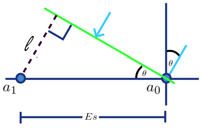
Figure 1: Impinging planar wave onto 2 antenna line array.

Modifying the phase of the received signals and adding them together allows us to create gains and nulls in specific directions. Because modifying the phase of complex signals is super easy, you just multiply by a complex number, nearly all beamformers convert the received signals to their complex baseband equivalents. Converting the received signals to their baseband equivalents can be accomplished through quadrature sampling or through Hilbert filtering, both of which are beyond the scope of this post.

We can now create something called the steering vector. The steering vector simply contains the phase offsets each antenna sees for a given signal propagating from some direction. In our two element example the steering vector is $s(\phi) = [1,e^{-j\phi}]^T$ where $T$ represents transpose. Notice that for the first antenna there is no phase offset. This is because we are computing all offsets with respect to antenna $a_0$.

Block Diagram Setup

Now that we have a good understanding of how waves propagate through space and how the angle of propagation affects the phase at the receive antenna, let’s put together a block diagram of our system. Figure 2 shows our system containing a signal of interest (SOI), which is the signal we are trying to receive, and an interferer that is making it hard to sense the SOI. The blocks $C_{soi x}$ and $C_{i x}$ represent the channel through which the SOI and interferer signals travel in order to reach antenna x. Notice that the received signal comprises three components, the SOI, the interferer, and some white noise. Note that we assume the three components are uncorrelated with one another. The phases of the received signal are modified by multiplying by a complex weight and then summed together. Notice that the complex weight is conjugated before being applied to the received signal.

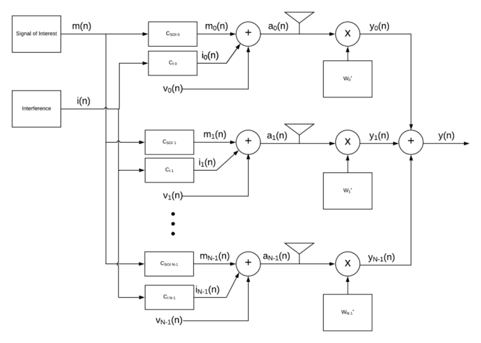
Figure 2: Adaptive beamforming block diagram

Adaptive Beamforming Setup

The way to think about setting up the problem is that we want to find the weights that minimize the average power in $y$ while preserving the power emanating from our SOI. Average power is computed by $E\{|y|^2\}$ or $E\{\mathbf{w}^H \mathbf{aa}^H \mathbf{w}\}$ in vector form where $E\{\}$ is the expectation operator which returns the expected value, think average, of a random variable, and $H$ is the Hermitian operator. To preserve our SOI we can set $\mathbf{w}^H \mathbf{s}_{SOI} = 1$, which is essentially saying that all signals propagating from the same angle as our SOI experience unity gain.

We have all the elements of a constrained optimization problem which can be written as

$$\underset{\mathbf{w}^H}{\arg\min}\{E\{\mathbf{w}^H \mathbf{a}\mathbf{a}^H \mathbf{w}\} \}  \quad \text{s.t.} \quad \mathbf{w}^H \mathbf{s}(\phi) =1\\$$

which simplifies to
\begin{align*}
\underset{\mathbf{w}^H}{\arg\min}\{\mathbf{w}^H \mathbf{R}_a\mathbf{w} \} \quad \text{s.t.} \quad \mathbf{w}^H \mathbf{s}(\phi) =1\\
\end{align*}

where $\mathbf{R}$ is the spatial correlation matrix of received samples.

This constrained optimization problem can be solved using Lagrange multipliers. Using Lagrange multiplies is a little beyond the scope of this short tutorial but the solution can be easily understood without the diving into Lagrange multipliers. The weights that minimize the average power while still maintaining gain in the in the direction of the SOI is given by

\begin{align*}
\mathbf{w} = \frac{\mathbf{R}_a^{-1}\mathbf{s}(\phi)}{ \mathbf{s}^H(\phi) \mathbf{R}_a^{-1}\mathbf{s}(\phi)}.
\end{align*}

The numerator is simply the steering vector (the vector containing the phase offsets for a signal propagating in a desired direction) multipliedd by the inverse of the spatial correlation matrix. This creates a vector of weights that's then scaled by the denominator. This solution produces the minimum variance distortionless response (MVDR) beamformer. While the name is a bit of a mouthful it can be broken into two parts to understand. Minimum variance refers to minimizing the power at the output of the beamformer. Remember, the power of a random variable is related to its variance and so minimum variance means smallest power. Distortionless response refers to the fact that the power of the SOI remains the same, it is not attenuated nor gained by going through the beamformer.

MVDR Scanning Vector

The last step needed to understand and make sense of beamformers is to create the scanning vector. In truth, the scanning vector is commonly used for one of two purposes, visualizing the spatial gain pattern of the apparent antenna and getting an estimate of the angle of arrival (AoA) of an interferer. Scanning vectors are very similar to steering vectors in fact, they are computed in the same way. The difference is scanning vectors sweep the AoA instead of focusing on only the AoA of the SOI.  Another difference is that scanning vectors are not used to compute the weights of the adaptive beamformer, only the steering vector is used in finding the weights.

To get the gain in a given direction all you need to do is compute the scanning vector for that direction and perform a dot product between the adaptive beamforming weights and the scanning vector. In other words, if $\mathbf{h} = [1, e^{-j\beta}]^T$ where $\beta$ is the phase offset corresponding to signals propagating from the direction you wish to find the gain for, then the gain is found by $\mathbf{w}^H\mathbf{h}$.

Figure 3 shows the spatial gain response of an apparent antenna for an MVDR beamformer with 6 antennas spaced at a half wavelength apart. The SOI's AoA is 90 degrees while the interferer's AoA is 10 degrees. Notice that the MVDR places a deep null in the direction of the interferer while preserving the energy emitted from the direction of the SOI.

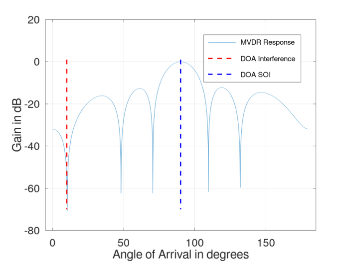
Figure 3: MVDR spatial response using a six-element antenna with an inter-element spacing of half a wavelength. Interference is at 10 degrees with SOI at 90 degrees.

Figure 4 uses the same setup but shows the MVDR spatial gain response for a second interferer placed at 120 degrees. Notice that the gain response adapts to the new circumstance (hence this is an adaptive beamformer).

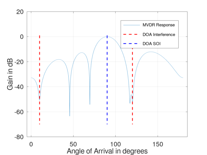
Figure 4: MVDR spatial response using a six-element antenna with an inter-element spacing of half a wavelength. Interference is at 10 degrees and 120 degrees with SOI at 90 degrees.

Conclusion

Adaptive beamformers are powerful tools used to mitigate unwanted interference. However, those considering the use of adaptive beamformers should be aware of a few complexities. The first is that the adaptive beamformers must know the precise location of each antenna as this affects the steering vector. Second, adaptive beamformers require the user to know which direction the SOI is coming from. If this is not precisely known, the adaptive beamformer may try to place a null in the direction of the SOI. For stationary platforms this might not be much of an issue, especially if the direction of the SOI does not move. However, if on a moving and rotating platform, this can be very difficult, involving more sensors to obtain an accurate estimate of the platform's orientation.

If the SOI is below the noise floor, then the design could be greatly simplified by using a nuller instead of a beamformer like the one shown here. Nullers do not maintain gain in any direction, they simply try to take out power emanating from any direction, hence the SOI needs to be below the noise floor for this approach to be considered. However, the nuller needs no information about the orientation of the platform, the direction of the SOI, nor precise information about it's antenna locations.

Finally, the number of interferers an adaptive beamformer can remove is estimated to be N-1 where N is the number of antenna elements in the system. Sometimes you can get lucky and a sympathetic null takes one out but that can't be controlled nor relied on. Sympathetic nulls are the nulls created by the adaptive beamformer that are unintended, such as the null at 48 degrees in Figure 3. Lastly, if an interferer is coming from the same direction as the SOI then you can't spatially remove the interference.

While adaptive beamformers do increase the complexity of the system, they should be strongly considered if the interference prevents your system from recovering the SOI. Please list your comments and questions below or point out mistakes.

Sign in