Off-Topic: A Fluidic Model of the Universe

Cedron Dawg●February 2, 2022●6 comments

Academia / Research

Introduction

This article is a followup to my previous article "Off Topic: Refraction in a Varying Medium"[1]. Many of the concepts should be quite familiar and of interest to the readership of this site. In the "Speculations" section of my previous article, I mention the goal of finding a similar differential equation as (18) of [1] for light traveling in gravity. It turns out it is the right equation, but a wrong understanding. As a consequence of trying to solve this puzzle, a new hypothesis for gravity arose with a similar differential equation to use for massive particles. One thing leads to another, and seeking an explanation for mass leads to a new model of the foundational layer of reality. The model is purely fluidic. That is, reality seems to be formed out of a fluid, its flows, and compression waves.

The ingredients for this thesis are one premise, one conjecture, one empirical correction, and the rest is either mathematics or deductive reasoning. It goes from solid to speculative. The latter starting pretty much where the math stops. Those sections can be considered a to-do list mathematically and they should be able to validate or invalidate the conjectures. It is fluid dynamics modeling so it is complicated and computational intensive and a rich field for specialized numerical techniques.

Though this is a speculative hypothesis, it is presented as being factually true in order to reduce the tremendous number of qualifiers that would be necessary. It has passed more thought experiments than included in this article, and has not failed any. Optimistically, it appears to have the potential to answer many of today's unsolved mysteries. However, it does contradict General Relativity (GR); they both can't be correct.

This article is available in PDF format for easy printing

The first part of this article is like my others: A derivation of a formula along with an explanation. The math should be able to stand on its own. Whether or not it ends up being an accurate description of reality remains to be seen. Whichever the case, it is still a lot of cool math, and can hopefully serve as a learning tool. The second half is more descriptive, with hopefully math to follow some day.

Newtonian Spoken Here

The good news for many is that the theory is rooted in good old Newtonian coordinates with no need to mix the time coordinate with any space coordinates for some sort of frame of reference transformations. This is known as "3D+T", three dimensions and time. No extra dimensions are needed. The equations mostly have common sense relatable conceptualizations. The objective perspective is employed. It doesn't care whether an observer is watching, it works how it works. Any observation techniques that interferes can also be described objectively.

Even better news for others is that there are no complex values in any of the quantities in this article. The math is largely high school level, requiring a knowledge of vectors, dot products, and gradients. Some Calculus is also used. All values are real valued.

The Speed Equation

Consider the classic example of refraction where a beam of light is being bent by the surface of water, or the surface of a hunk of glass. The index of refractions ($n$) of the materials at the surface boundary are used along with Snell's law to do angle calculations. It is explained that Snell's law works because the light is slowed down more by the material with the higher index of refraction.

$$ \left\| \vec v \right\| = \frac{L}{n} \tag{1} $$

Usually '$c$' is the variable name used in the numerator on the right side, including in my previous article. The letter '$L$' is being used instead because there is some ambiguity in how '$c$' is defined. Traditionally, the value of '$n$' is real and never goes below one, and is one in completely empty space. Completely empty space actually doesn't exist, so light never reaches the full 'vacuum speed'. Apparent less than one, or even zero, values of $n$ and complex values are not considered in this article. Like the previous article, it is an ideal theoretical treatment.

Refraction in a Varying Media

Often, marching soldiers or toy trucks are used to demonstrate the bending at the boundary. The examples are usually presented as though the light makes a sharp corner at the surface. If one considers the object of refraction being a point particle and knowing that sharp corners can't occur in nature, there should be a curved trajectory that is describable by a vector differential equation.

In the refraction of light, the photon is always trying to turn into the higher index of refraction. Therefore its acceleration at any point has to lay in the plane defined by the velocity and the gradient of the index of refraction. This is (16) from [1], converted back into index of refraction terms.

$$ \begin{aligned} \dot{\vec v} &= \left( \frac{ \vec v \cdot \vec v }{n} \right) \vec{\nabla} n - \frac{2}{n} \left( \vec{\nabla}n \cdot \vec v \right) \vec v \\ &= \left( \vec v \cdot \vec v \right) \frac{\vec{\nabla} n}{n} - 2 \left( \frac{\vec{\nabla} n}{n} \cdot \vec v \right) \vec v \\ \end{aligned} \tag{2} $$

The second line puts the equation in a form where the gradient has been normalized by the index of refraction.

Fluff Density

By taking the natural logarithm, the $1$ based index of refraction scale is transformed to a $0$ based scale, where the zero represents the empty vacuum situation. The higher the value, the slower the speed, so it is easy to visualize this value as a resistance measure. In my first article I called it 'fluff', and its measure was density. The denser the fluff, the slower the refractive particle can move through it.

$$ \rho = \ln(n) \tag{3} $$

The speed of the refractive particle can now be expressed solely in terms of the maximum possible speed and the local fluff density.

$$ \left\| \vec v \right\| = L e^{-\rho } \tag{4} $$

The gradient of the fluff density will lay in the same direction as the gradient of the index of refraction. The rescaling turns out to be exactly the same as the normalized form above.

$$ \vec{\nabla} \rho = \frac{\vec{\nabla} n}{n} \tag{5} $$

The vector differential form of Snell's Law can then be expressed in terms of the fluff density gradient. Notice that the fluff density itself $\rho$ and the maximum possible speed limit $L$ are not in the equation. Of course they are still there implicitly in the form of the magnitude of $\vec v$. This will be called the "steering equation".

$$ \begin{aligned}\label{RefractiveSteering} \dot{\vec v} &= \left( \vec v \cdot \vec v \right) \vec{\nabla} \rho - 2 \left( \vec{\nabla} \rho \cdot \vec v \right) \vec v \\ \end{aligned} \tag{6} $$

This equation has many remarkable properties, of which some will be revealed in the treatment that follows. Its derivation is shown in my previous article.[1]

The Refractive Particle Steering Equation

The steering equation has two terms. The first is independent of the direction of velocity and the other is. Therefore, the first can be seen as an acceleration all refractive particles have in a fluff gradient and the second as a direction dependent adjustment.

When the trajectory is orthogonal to the fluff gradient, the dot product in the second term is zero and there is no adjustment. The acceleration is entirely in the direction of the gradient.

When the trajectory is along the fluff gradient, the dot product reaches its extreme value, and the second term becomes exactly twice the negative of the first term. The net result is the acceleration is now entirely opposite the direction of the gradient with the same magnitude since it is simply the negative.

At angles in between there will be some acceleration along the trajectory as well. For trajectories at 45 degrees to the horizon, in either direction, the acceleration will be entirely along the transverse.

When the $\left(\vec{\nabla} \rho \cdot \vec v\right)$ dot product is positive, it means the refractive particle is heading into thicker fluff and thus slowing down along the trajectory. Conversely, when the dot product is negative, it means the trajectory is heading out of the thicker fluff and able to speed up so its acceleration is positive along the trajectory.

The magnitude of both terms is quadratic with the magnitude of velocity and linear with the magnitude of the fluff gradient. This means the whole equation is. The linearity of the fluff gradient is the greatest advantage of working on the logarithmic fluff density scale rather than the base index of refraction scale.

Express with Unit Vectors

The gradient and velocity vectors can be expressed with their magnitudes and directions separated by defining a unit direction vector for each.

$$ \begin{aligned} \vec u_\rho = \frac{ \vec{\nabla} \rho }{ \left\| \vec{\nabla} \rho \right\| } &\to \vec{\nabla} \rho = \left\| \vec{\nabla} \rho \right\| \vec u_\rho \\ \end{aligned} \tag{7} $$ $$ \begin{aligned} \vec u_v = \frac{ \vec v }{ \left\| \vec v \right\| } &\to \vec v = \left\| \vec v \right\| \cdot \vec u_v \\ \end{aligned} \tag{8} $$

The vectors are then seen as magnitude times direction, or if you prefer, magnitude in a direction. The steering equation can then be rewritten to be magnitude and direction separable.

$$ \begin{aligned}\label{AccelerationVector} \dot{\vec v} &= \left( \vec v \cdot \vec v \right) \vec{\nabla} \rho - 2 \left( \vec{\nabla} \rho \cdot \vec v \right) \vec v \\ &= \left\| \vec v \right\|^2 \left\| \vec{\nabla} \rho \right\| \left[ \vec u_\rho - 2 \left( \vec u_\rho \cdot \vec u_v \right) \vec u_v \right] \\ &= L^2 e^{ -2\rho } \left\| \vec{\nabla} \rho \right\| \vec u_a = \left\| \dot{\vec v} \right\| \vec u_a \\ \end{aligned} \tag{9} $$

The Direction is Magnitude Independent

The unit vector for the acceleration direction was implicitly defined in the prior equation as this:

$$ \vec u_a = \vec u_\rho - 2 \left( \vec u_\rho \cdot \vec u_v \right) \vec u_v \tag{10} $$

It is easily proved that the vector has length one and is thus appropriately labeled as unit vector.

$$ \begin{aligned} \vec u_a \cdot \vec u_a &= \left[ \vec u_\rho - 2 \left( \vec u_\rho \cdot \vec u_v \right) \vec u_v \right] \cdot \left[ \vec u_\rho - 2 \left( \vec u_\rho \cdot \vec u_v \right) \vec u_v \right] \\ &= \vec u_\rho \cdot \vec u_\rho - 4 \left( \vec u_\rho \cdot \vec u_v \right) \vec u_\rho \cdot \vec u_v + 4 \left( \vec u_\rho \cdot \vec u_v \right)^2 \vec u_v \cdot \vec u_v \\ &= 1 - 4 \left( \vec u_\rho \cdot \vec u_v \right)^2 + 4 \left( \vec u_\rho \cdot \vec u_v \right)^2 \cdot 1 \\ &= 1 \\ \end{aligned} \tag{11} $$

This means that the direction of the acceleration is only dependent on the directions of the velocity and fluff density gradient, not their magnitudes. They don't appear in the equation, only the unit direction vectors do.

The Magnitudes are Direction Independent

The magnitudes, in a similar manner, are independent of the direction. They are dependent only on the fluff density. For the velocity, that is already part of the premise definition.

$$ \left\| \vec v \right\| = L e^{ -\rho } \tag{12} $$

So the speed (magnitude of velocity) is the same no matter which direction the refractive particle is traveling. This is also true for the acceleration. From ():

$$ \begin{aligned} \left\| \dot{\vec v} \right\| &= \left\| \vec v \right\|^2 \left\| \vec{\nabla} \rho \right\| = \left( L e^{ -\rho } \right)^2 \left\| \vec{\nabla} \rho \right\| = L^2 e^{ -2\rho } \left\| \vec{\nabla} \rho \right\| \\ \end{aligned} \tag{13} $$

The magnitude of the acceleration is not only dependent on the fluff density, but it is also linearly dependent on the magnitude of the fluff gradient. It is very easy to see from this equation, that in a region of constant fluff density where the gradient is zero, there is no acceleration felt and the particle will travel with a constant velocity.

Permittivity and Permeability

The speed of light in a true vacuum, aka free space, is usually given by:

$$ c_0 = \frac{1}{ \sqrt{\epsilon_0 \mu_0} } \tag{14} $$

Where $\epsilon_0$ is electric permittivity and $\mu_0$ is magnetic permeability in a gravity free true vacuum. From a universal perspective, the speed of light near a massive object slows down. Therefore, one of the values of $\epsilon$ or $\mu$ must be changing, or both. The equation is then rewritten without the naught subscripts to indicate variable values.

$$ c = \frac{1}{ \sqrt{\epsilon \mu} } = \| \vec v \| = \frac{L}{n} \tag{15} $$

With appropriately chosen units the value of $L$ can be set to one. Its actual value has no qualitative bearing on the behavior of the equations and there is price paid for dropping the variable name in the ability to track the units, so it is retained.

Cross multiplying the outer terms gives a formula for then index of refraction in terms of the two fields.

$$ n = L \sqrt{\epsilon \mu} \tag{16} $$

Taking the log of both sides to get the fluff density isolates the limit speed in its own term.

$$ \rho = \ln(n) = \ln(L) + \frac{ \ln(\epsilon) + \ln(\mu)}{2} \tag{17} $$

As a result, the gradient is independent of the limit speed.

$$ \vec{\nabla}\rho = \frac{\vec{\nabla} n }{n} = \frac{1}{2} \left( \frac{ \vec{\nabla} \epsilon }{\epsilon} + \frac{ \vec{\nabla} \mu }{ \mu} \right) \tag{18} $$

For a central point source, there doesn't seem to be any doubt that $\vec{\nabla} \epsilon$ and $\vec{\nabla} \mu$ would be collinear along a radial. Is this a true in general? Irrelevant to this discussion. What if relevant is that an alternative definition of the gradient of the fluff density has been made using two well known fields from physics.

This definition of $\vec{\nabla} \rho$ can then be plugged into the steering equation and separated into two parts.

$$ \begin{aligned} \dot{\vec v} &= \left( \vec v \cdot \vec v \right) \vec{\nabla} \rho - 2 \left( \vec{\nabla} \rho \cdot \vec v \right) \vec v \\ &= \frac{ \left[ \left( \vec v \cdot \vec v \right) \frac{ \vec{\nabla} \epsilon }{\epsilon} - 2 \left( \frac{ \vec{\nabla} \epsilon }{\epsilon} \cdot \vec v \right) \vec v\right] +\left[ \left( \vec v \cdot \vec v \right) \frac{ \vec{\nabla} \mu }{\mu} - 2 \left( \frac{ \vec{\nabla} \mu }{\mu} \cdot \vec v \right) \vec v\right] }{2} \\ &= \frac{ \dot{\vec {v}}_\epsilon + \dot{\vec {v}}_\mu }{2} \end{aligned} \tag{19} $$

The definition of these two parts come from the partitioning.

$$ \begin{aligned} \dot{\vec {v}}_\epsilon &= \left( \vec v \cdot \vec v \right) \frac{ \vec{\nabla} \epsilon }{\epsilon} - 2 \left( \frac{ \vec{\nabla} \epsilon }{\epsilon} \cdot \vec v \right) \vec v \\ \dot{\vec {v}}_\mu &= \left( \vec v \cdot \vec v \right) \frac{ \vec{\nabla} \mu }{\mu} - 2 \left( \frac{ \vec{\nabla} \mu }{\mu} \cdot \vec v \right) \vec v \\ \end{aligned} \tag{20} $$

Since each of the fields obeys the steering equation, they are by definition refractive in behavior. Whether these fields are independent or not, it is the composite value, the index of refraction, that is the only value needed to define behavior of photons presumed to be behaving refractively.

Central Source Point Model

A central source point model is very useful in Physics to model finite objects. The model is understood to be a representation which provides useful description. The mathematics for a single point is generally much simpler than dealing with a spacial object. Point models are simple ideals that lay the foundation for more sophisticated models to explain observed deviations from the simpler ideal.

To explain the curvature of the trajectory of a photon passing by the sun, an ideal model of an index of refraction distribution is used for the sun and a refractive particle is used for the photon.

It turns out that the model I conjectured in my previous article [1] coincides with the "far-field approximation" (12) found by Ye and Lin in [2], though their version also comes with a value for $k$.

$$ \begin{aligned} n &= \exp \left(- \frac{2P_r}{c^2} \right) \\ P_r &= - \frac{GM}{r} \\ \end{aligned} \tag{21} $$

The speed of light in a pure vacuum is:

$$ c = c_0 = L \tag{22} $$

Which makes the index of refraction definable as:

$$ n = \exp \left( \frac{2GM}{L^2r} \right) = e^{ \frac{k}{r} } \tag{23} $$

Where $k$ is implicitly defined as:

$$ k = \frac{2GM}{L^2} \tag{24} $$

This $k$ value represents the strength of the index of refraction field surrounding the central point source.

By definition, Ye and Lin's formula is empirically correct in the far field region. The conjecture in my prior article, and maintained in this one, is that it is actually the true theoretical description even in the near field of massive objects.

Black Holes Aren't Possible

Whether or not a black hole is possible is based on the distribution model used for the index of refraction values around a central source point. Various models are compared in the appendices. Using this model, black holes aren't possible. Other models, including GR which does allow for them, are shown in the appendices.

Defining the index of refraction at every point in space also defines the speed of the refractive particle at that point. The formula for the field becomes:

$$ \| \vec v \| = \frac{L}{n} = L e^{ - \frac{2GM}{L^2r}} = L e^{ -\frac{k}{r} } \tag{25} $$

Notice that for every value of $r$ that is not zero, the speed cannot be zero. As a refractive particle approaches the center point, it slows down, but never stops. Of course, a real black hole would have a physical radius so this region could never be reached. As the refractive particle moves away, its speed increases towards the limit value of free space.

$$ \begin{aligned} \lim_{r \to 0} \| \vec v \| = 0 \\ \lim_{r \to \infty} \| \vec v \| = L \\ \end{aligned} \tag{26} $$

Convert to a Fluff Scale

As noted in my previous article, and Ye and Lin in [2], working in the log scale is a lot easier as far as the math goes.

$$ \rho = \ln(n) =\frac{k}{r} \tag{27} $$

The gradient is always pointing inward and its magnitude follows the inverse square law.

$$ \vec{\nabla} \rho = -\frac{k}{r^2} \vec u_r \tag{28} $$

Plugging in the value of $k$ given by Ye and Lin (24) connects the fluff density gradient to the mass of the central point.

$$ \vec{\nabla} \rho = -\frac{2GM}{L^2r^2} \vec u_r \tag{29} $$

Notice the similarity to the Newtonian gravitational potential. The different sign convention does not impact the behavior.

$$ \Phi = -\frac{GM}{r} \tag{30} $$

The gradient is always pointing outward, and another sign convention is used to call gravity inward.

$$ \vec{\nabla} \Phi = \frac{GM}{r^2} \vec u_r = - \vec g \tag{31} $$

We come to the realization that the acceleration of the refractive particle is twice the strength of gravity.

$$ \vec{\nabla} \rho = -\frac{2}{L^2} \vec{\nabla} \Phi = \frac{2}{L^2} \vec g \tag{32} $$

That they are proportional is not surprising, since their potential functions are proportional. It is the value of two that counts. This value is shared among all the models compared in the appendices.

Newton's Gravitational Constant

When the magnitude of refractive acceleration is put in terms of the gravitational acceleration, something interesting happens.

$$ \begin{aligned} \left\| \dot{\vec v} \right\| &= \left\| \vec v \right\|^2 \cdot \left\| \vec{\nabla} \rho \right\| = \left\| \vec v \right\|^2 \frac{2GM/L^2}{r^2} \\ &= \frac{GM}{r^2} \cdot 2 \left( \frac{\left\| \vec v \right\|}{L} \right)^2 = \frac{GM}{r^2} \cdot 2 e^{-2\rho} = \frac{[Ge^{-2\rho}]M}{r^2} \cdot 2 \\ &= \frac{G'M}{r^2} \cdot 2 \\ \end{aligned} \tag{33} $$

Where

$$ G' = Ge^{-2\rho} \tag{34} $$

The trailing factor of '2' was expected, as the force bending of light around the sun is twice what is expected from gravity. However, the $G'$ indicates that Newton's constant varies when using universal coordinates. The ratio is the same as the ratio of the local speed of light to $L$ squared.

$$ \begin{aligned} \frac{G'}{G} &= \left( \frac{\left\| \vec v \right\|}{L} \right)^2 = e^{-2\rho} \\ \end{aligned} \tag{35} $$ $$ \begin{aligned} \frac{G'}{\left\| \vec v \right\|^2} &= \frac{G}{L^2} \\ \end{aligned} \tag{36} $$

This is kind of a big deal. It means in the universal coordinates being used, when regions of deeper gravity are considered from far away, Newton's constant isn't really constant. This ratio appears in several of the formulas and allows an immediate translation from universal to local coordinates.

Multiple Sources

When considering a real world problem, there are going to be multiple massive objects which define the fluff density. They will also likely be moving. That aspect is not covered in this article, but is a natural extension. When they are moving, the property of superposition no longer applies and the accelerations have to be calculated using relative velocities for each object and then summed.

In the case of multiple static objects, the field can be defined by simply summing the potentials. Since the gradient is a linear operator, the gradients can be summed too.

$$ \begin{aligned} \rho &= \sum_i \rho_i = \sum_i \frac{k_i}{r_i} = \frac{2G}{L^2} \sum_i \frac{M_i}{r_i} \\ \vec{\nabla} \rho &= \sum_i \vec{\nabla} \rho_i = -\sum_i \frac{k_i}{r_i^2} \vec{u}_{r,i} = -\frac{2G}{L^2} \sum_i \frac{M_i}{r_i^2} \vec{u}_{r,i} \\ \end{aligned} \tag{37} $$

Where

$$ \begin{aligned} \vec r_i &= \vec x - \vec x_i \\ r_i &= \| \vec r_i \| = \| \vec x - \vec x_i \| \\ r_i^2 &= \vec r_i \cdot \vec r_i \\ \vec{u}_{r,i} &= \frac{ \vec r_i }{ \| \vec r_i \| } = \frac{\vec x - \vec x_i}{ \| \vec x - \vec x_i \| } \\ \end{aligned} \tag{38} $$

These are the same operations that would be undertaken to calculate a Newtonian gravitational potential and gradient fields. The result is that for any point in space, the fluff density and the fluff density gradient can be calculated.

Equivalent Single Body

The inverse can be calculated for a single body, or an equivalent single body, can be calculated at any point where the gradient isn't zero. The magnitude of the fluff gradient can be found from (28).

$$ \| \vec{\nabla} \rho \| = \frac{k}{r^2} \tag{39} $$

Dividing (27) by (39) gives the equation for the equivalent radius.

$$ r =\frac{\rho}{\| \vec{\nabla} \rho \|} \tag{40} $$

Using (27) again, the equivalent strength parameter ($k$) can be found.

$$ k = \rho r =\frac{\rho^2}{\| \vec{\nabla} \rho \|} \tag{41} $$

The equivalence only exists at a single point in a multibody field. For regions near a dominant fluff source, these formulas will give an approximation to the objects properties. A more accurate measure would require several points and an estimate of the underlying fluff density field.

Of course, these formulas are based on (27) as the fluff density model around a central point. Other models are shown in the appendices and would have different formulas for these.

Refraction, not Gravity

This article assumes that it is refraction that is curving the trajectory of a photon as it passes the sun, not gravity. The behavior of the photon is as if gravity is acting on it when it is passing transversely to the gravity gradient, but if it is heading directly towards the sun it is slowing down. This means the acceleration is point away from the sun, opposite of what gravity would do. Refraction explains the behavior, gravity does not. As shown in the "Newton's Gravitational Constant" section above, the log of the index of refraction distribution, represented as a fluff density, is proportional to the Newtonian gravity field.

Gravitational Force

Let's assume that a stationary massive particle is a set of refractive particles orbiting around a central point in some sort of harness. Furthermore, suppose the harness is so small that both the fluff density and gradient can be considered constant in the region.

Different harness configurations and orientations can be considered. Suppose the harness is like a merry-go-round, and the refractive particles are spinning around and around with their axis aligned with the fluff gradient. Each refractive particle would feel the same acceleration as a transverse pass constantly, so the net effect is the same as a single particle exhibiting gravity at double strength. All the particles would be feeling a force in the same direction. However, if the harness is like a Ferris-wheel, the net accelerations will be zero! The net force generated traversely will be exactly opposed by the particles traveling radially. Therefore it is obvious that the net sum of acceleration of a harnessed set of refractive particles is dependent on the nature of the harness and orbits taken by the particles.

It is possible to calculate the net average of "orbits with every possible direction", by integrating using a sphere to define the input direction. Since the angles are independent of direction, the speed and magnitude of the gradient can be set to one without loss of generality.

The acceleration vector is set up as the average of all the output vectors.

$$ \vec a = \frac{\vec N}{D} = \frac{ \int_0^{2\pi} \int_0^{\pi} \vec u_a \sin(\phi) d\phi d\theta }{ \int_0^{2\pi} \int_0^{\pi} 1 \sin(\phi) d\phi d\theta } \tag{42} $$

The denominator is actually the surface area of the unit sphere.

$$ D = \int_0^{2\pi} \int_0^{\pi} 1 \sin(\phi) d\phi d\theta = 2\pi\left[ -\cos(\phi) \right]_0^{\pi} = 4\pi \tag{43} $$

A small local orthonormal coordinate system is set up. The input velocity is represented by a point on the sphere. Dropping a projection onto the horizontal plane gives a vector perpendicular to the radial laying in the XY plane.

$$ \vec u_{\perp} = \cos(\theta) \vec u_x + \sin(\theta) \vec u_y \tag{44} $$

The input velocity vector can then be defined in terms of the integrals variables.

$$ \begin{aligned} \vec u_v &= \cos(\phi) \vec u_\rho + \sin(\phi) \vec u_{\perp} \\ &= \cos(\phi) \vec u_\rho + \sin(\phi) \cos(\theta) \vec u_x + \sin(\phi) \sin(\theta) \vec u_y \\ \end{aligned} \tag{45} $$

Likewise with

$$ \vec u_\rho \cdot \vec u_v = \cos(\phi) \tag{46} $$

And the unit acceleration vector.

$$ \begin{aligned} \vec u_a &= \vec u_\rho - 2 \left( \vec u_\rho \cdot \vec u_v \right) \vec u_v \\ &= \vec u_\rho - 2 \cos(\phi) \left[ \cos(\phi) \vec u_\rho + \sin(\phi) \cos(\theta) \vec u_x + \sin(\phi) \sin(\theta) \vec u_y \right] \\ &= \left( 1 - 2 \cos^2(\phi) \right) \vec u_\rho - 2 \sin(\phi) \cos(\theta) \vec u_x - 2\sin(\phi) \sin(\theta) \vec u_y \\ \end{aligned} \tag{47} $$

The numerator can now be evaluated.

$$ \begin{aligned} \vec N &= \int_0^{2\pi} \int_0^{\pi} \vec u_a \sin(\phi) d\phi d\theta \\ &= \left( \int_0^{2\pi} \int_0^{\pi} \left( 1 - 2 \cos^2(\phi) \right) \sin(\phi) d\phi d\theta \right) \vec u_\rho + 0 \vec u_x + 0 \vec u_y\\ &= 2\pi \left[ -\cos(\phi) + \frac{ 2 }{3} \cos^3(\phi) \right]_0^{\pi} \vec u_\rho \\ &= 2\pi \left[ 2 - \frac{ 4 }{3} \right] \vec u_\rho \\ &= \frac{ 4 }{3}\pi \vec u_\rho \\ \end{aligned} \tag{48} $$

Finally, the average acceleration can be calculated.

$$ \vec a = \frac{\frac{ 4 }{3}\pi \vec u_\rho}{ 4\pi } = \frac{1}{3} \vec u_\rho \tag{49} $$

This was not expected. The desired result should have a half, not a third. This is a whole number discrepancy, not just some margin of error thing, so there has to be a rule based answer.

Motion Enhanced Gravitational Acceleration

Suppose that the massive particle is moving, rather than being stationary, and that this movement is slow in comparison to the speed of the refractive particles in the harness. The velocity for any of the refractive particles in any point in their orbits can be decomposed into a harness velocity ($\vec h$) and the massive particle's velocity ($\vec d$).

$$ \vec v = \vec h + \vec d \tag{50} $$

A couple of dot products will be needed.

$$ \begin{aligned} \vec v \cdot \vec v &= \vec h \cdot \vec h + 2 \left( \vec h \cdot \vec d \right) + \vec d \cdot \vec d \\ \vec{\nabla} \rho \cdot \vec v &= \vec{\nabla} \rho \cdot \vec h + \vec{\nabla} \rho \cdot \vec d \\ \end{aligned} \tag{51} $$

The composite velocity (50) can then be inserted into the steering equation ().

$$ \begin{aligned} \dot{\vec v} &= \left( \vec v \cdot \vec v \right) \vec{\nabla} \rho - 2 \left( \vec{\nabla} \rho \cdot \vec v \right) \vec v \\ &= \left( \vec h \cdot \vec h + 2 \left( \vec h \cdot \vec d \right) + \vec d \cdot \vec d \right) \vec{\nabla} \rho - 2 \left( \vec{\nabla} \rho \cdot \vec h + \vec{\nabla} \rho \cdot \vec d \right) \left[\vec h + \vec d \right]\\ &= \left( \vec h \cdot \vec h \right) \vec{\nabla} \rho - 2 \left( \vec{\nabla} \rho \cdot \vec h \right) \vec h \\ & + 2 \left( \vec h \cdot \vec d \right) \vec{\nabla} \rho - 2 \left( \vec{\nabla} \rho \cdot \vec d \right) \vec h - 2 \left( \vec{\nabla} \rho \cdot \vec h \right) \vec d \\ & + \left( \vec d \cdot \vec d \right) \vec{\nabla} \rho - 2 \left( \vec{\nabla} \rho \cdot \vec d \right) \vec d \\ &= \dot{\vec v}_h + 2 \left[ \left( \vec h \cdot \vec d \right) \vec{\nabla} \rho - \left( \vec{\nabla} \rho \cdot \vec d \right) \vec h - \left( \vec{\nabla} \rho \cdot \vec h \right) \vec d \right] + \dot{\vec v}_d \\ \end{aligned} \tag{52} $$

When this acceleration definition is run through the same spherical averaging as in the previous section, another remarkable thing happens. The three mixed terms zero out and the result is that the net accelerations are separated and additive.

$$ \vec a = \frac{ \int_0^{2\pi} \int_0^{\pi} \dot{\vec v} \sin(\phi) d\phi d\theta }{ \int_0^{2\pi} \int_0^{\pi} 1 \sin(\phi) d\phi d\theta } = \vec a_h + \vec a_d \tag{53} $$

The first term is the acceleration due to the harness ($\vec a_h$), which is the same as the previous section, except the speed is retained. The second term is the acceleration ($\vec a_d$) due to the massive particle's motion relative to the fluff/gravity field. Since these are vectors, there is also a directional aspect. The accelerations here, denoted with $\vec a$, are the net accelerations of the massive particle while the $\dot{\vec v}$ variables are the instantaneous accelerations of a constituent refractive particle.

The harness acceleration is the same as the static gravitational acceleration would be. Therefore the acceleration due to the displacement velocity can be said to be an enhancement to the acceleration.

The Massive Particle Steering Equation

Since there is a discrepancy between the speed equation premise (1) and empirical results from very accurate measurements, it is likely the premise is going to have to be modified rather than ignoring fundamental results. The two cases can be represented simultaneously by introducing a variable ($\lambda$) to stand for the ratio of refractive acceleration to gravitational acceleration on a transverse trajectory of a massive body.

The harness acceleration is then proportional to the square of the harness speed and adjusted with the $\lambda$ factor. In simple terms, perhaps intuitively, the harness speed $\|\vec h\|$ shouldn't be faster than $\| \vec v \| - \| \vec d \|$, so the parts of the orbit when $\vec d$ and $\vec h$ align, the sum shouldn't exceed the local speed of light, $\|\vec v\|$. The math can be worked that way, however, the math works much better, when a Pythagorean difference is applied instead. Since the harness speed already appears to be faster than the local speed of light because of the 1/3 to 1/2 discrepancy, it shouldn't really hurt to assume this limit instead. This is a loose end that needs further exploration.

The acceleration due to the displacement motion is entirely refractive in nature.

$$ \begin{aligned} \vec a_h &= \frac{\| \vec h \|^2}{\lambda} \vec{\nabla} \rho =\frac{ \| \vec v \|^2 - \| \vec d \|^2 }{\lambda} \vec{\nabla} \rho \\ \vec a_d &= \dot{\vec v}_d = \left( \vec d \cdot \vec d \right) \vec{\nabla} \rho - 2 \left( \vec{\nabla} \rho \cdot \vec d \right) \vec d \\ \end{aligned} \tag{54} $$

Both acceleration feature the fluff gradient. It can be expressed in terms of local gravity from (35) and the local speed of light. The displacement velocity can also be normalized to the local speed of light.

$$ \vec{\nabla} \rho = \frac{\lambda}{\| \vec v \|^2} \vec g \text{ and } \vec D = \frac{\vec d}{\| \vec v \|} \tag{55} $$

This makes the accelerations now described by gravity and the normalized displacement velocity.

$$ \begin{aligned} \vec a_h &= \left( 1 - \left( \vec D \cdot \vec D \right) \right) \vec g \\ \vec a_d &= \lambda \left[ \left( \vec D \cdot \vec D \right) \vec g - 2 \left( \vec g \cdot \vec D \right) \vec D \right] \\ \end{aligned} \tag{56} $$

The net acceleration is the sum of the two accelerations and the terms can combine to form a steering equation for a massive particle.

$$ \begin{aligned} \vec a &= \vec a_h + \vec a_d \\ &= \left[ 1 - \left( \vec D \cdot \vec D \right) \right] \vec g + \lambda \left[ \left( \vec D \cdot \vec D \right) \vec g - 2 \left( \vec g \cdot \vec D \right) \vec D \right] \\ &= \left[ 1 + ( \lambda - 1 ) \left( \vec D \cdot \vec D \right) \right] \vec g - 2 \lambda \left( \vec g \cdot \vec D \right) \vec D \\ \end{aligned} \tag{57} $$

If $\|\vec D\| = 0$, then it is straight up Newtonian gravity. If $\|\vec D\| = 1$, that is the object is traveling at the local speed of light, then the equation becomes the steering equation for a refractive particle. This is true independent of the value of $\lambda$.

At this point, it will be too cumbersome to carry $\lambda$ forward any further. Setting it to 2, an empirical match vs a premise match, means the premise need a little modification and the refractive particles in the harness somehow behave according to a variation, to be determined, of (1). The rest of the formulas can be worked for either value, 2 is assumed correct. Then the massive particle steering equation simplifies to:

$$ \begin{aligned} \vec a &= \left[ 1 + \left( \vec D \cdot \vec D \right) \right] \cdot \vec g - 4 \left( \vec g \cdot \vec D \right) \vec D \\ \end{aligned} \tag{58} $$

This vector differential equation describes the trajectory of a massive particle in a gravity field. Except for its refractive special case ($\|\vec D\|=1$), the magnitude of acceleration is direction dependent.

Sliding Sideways

One possible modification to the speed equation premise for refractive particles in a harness is to suggest that maybe they are also going sideways, and the speed equation only limits forward speed. Then, in order to resolve the discrepancy, that would mean that $\|\vec h\| = \sqrt{3/2} \|\vec v\|$, which means the harness speed is about 22\% faster than the local light speed. The sideways speed would be $\sqrt{5}/2 \|\vec v\|$, which has a "Golden Ratio" hint to it. Again, since this is a whole number discrepancy, it suggests that there is a fundamental principle at play, that can be mathematically described, and has an analytical solution.

Comparison to Relativistic Mass

One of the distinguishing features of General Relativity (GR) is that mass appears to increase when a massive object is in motion. The equation for the resultant mass, known as relativistic mass, is this:

$$ m = m_0 \frac{1}{ \sqrt{ 1 - \left(\frac{v}{c}\right)^2 } } \tag{59} $$

Since this is a scalar equation, it is direction independent. This effect can either be considered a change in mass, or the ratio of masses can be calculated and the RHS be considered an increase in gravitational acceleration instead. The two interpretations are mathematically identical.

$$ \begin{aligned} \frac{m}{ m_0 } &= \frac{1}{ \sqrt{ 1 - D^2 } } = \left(1-D^2 \right)^{-1/2} \\ &\approx 1 - \frac{1}{2} \left(-D^2\right) + \frac{3}{8} \left(-D^2\right)^{2} - \frac{5}{16} \left(-D^2\right)^{3} \\ &= 1 + \frac{1}{2} D^2 + \frac{3}{8} D^4 + \frac{5}{16} D^6 \\ &\approx 1 + \frac{1}{2} D^2 \\ \end{aligned} \tag{60} $$

For small value of $D$, this result is half of what the massive particle steering equation (58) predicts. In order to make this match the massive steering equation (57) the value of $\lambda$ would have to be $3/2$. This would cause a mismatch to GR's, and the empirical data, for a photon's travel past the sun. Therefore, GR is incompatible with the thesis of this article.

Steering in Polar Coordinates

In order to work in polar coordinates an appropriate set of unit vectors is helpful. The obvious candidates are a unit vector along the radial and an orthogonal one in the transverse direction. In this case a 2D model is being used.

$$ \begin{aligned} \vec u_r &= \left[ \cos(\theta), \sin(\theta) \right] \\ \vec u_{\theta} &= \left[ -\sin(\theta), \cos(\theta) \right] \\ \end{aligned} \tag{61} $$

These can be differentiated with respect to time.

$$ \begin{aligned} \dot{\vec u}_r &= \left[ -\sin(\theta), \cos(\theta) \right] \dot{\theta} = \dot{\theta}\vec u_{\theta} \\ \dot{\vec u}_{\theta} &= \left[ -\cos(\theta), -\sin(\theta) \right] \dot{\theta} = - \dot{\theta}\vec u_r \\ \end{aligned} \tag{62} $$

A general description of the position, velocity, and acceleration is then possible in terms of the unit vectors.

$$ \begin{aligned} \vec x &= r \vec u_r \\ \dot{\vec x} &= \dot{r} \vec u_r + r \dot{\theta} \vec u_{\theta} \\ \ddot{\vec x} &= \left( \ddot{r} - r \dot{\theta}^2 \right) \vec u_r + \left( 2 \dot{r} \dot{\theta} + r \ddot{\theta} \right) \vec u_{\theta} \\ \end{aligned} \tag{63} $$

The terms in the massive particle steering equation can also be expressed in polar terms.

$$ \begin{aligned} \vec D &= \frac{ \dot{\vec x} }{\| \vec v \| } = \frac{ \dot{r} \vec u_r + r \dot{\theta} \vec u_{\theta} }{\| \vec v \| } \\ \vec D \cdot \vec D &= \frac{ \dot{r}^2 + \left( r \dot{\theta} \right)^2 }{\| \vec v \|^2 } \\ \vec g &= -\frac{G'M}{r^2} \vec u_r \\ \vec g \cdot \vec D &= -\frac{G'M\dot{r}}{r^2\| \vec v \|} \\ \end{aligned} \tag{64} $$

Finally, the pieces can be put together and the polar form of the steering equation produced.

$$ \begin{aligned} \vec a &= \left[ 1 + \left( \vec D \cdot \vec D \right) \right] \vec g - 4 \left( \vec g \cdot \vec D \right) \vec D \\ &= -\frac{G'M}{r^2} \left[ \left( 1 + \frac{ \dot{r}^2 + \left( r \dot{\theta} \right)^2 }{\| \vec v \|^2 } \right) \vec u_r - 4 \frac{\dot{r}}{\| \vec v \|} \frac{ \left( \dot{r} \vec u_r + r \dot{\theta} \vec u_{\theta} \right) }{\| \vec v \|} \right] \\ &= -\frac{G'M}{r^2} \left[ \left( 1 + \frac{ -3 \dot{r}^2 + \left( r \dot{\theta} \right)^2 }{\| \vec v \|^2 } \right) \vec u_r - 4 \left( \frac{ \dot{r} r \dot{\theta} }{\| \vec v \|^2 } \right) \vec u_{\theta} \right] \\ &= -\frac{G'M}{\| \vec v \|^2 r^2} \left[ \left( \| \vec v \|^2 -3 \dot{r}^2 + \left( r \dot{\theta} \right)^2 \right) \vec u_r - 4 \left( \dot{r} r \dot{\theta} \right) \vec u_{\theta} \right] \\ \end{aligned} \tag{65} $$

It is not nearly as elegant in this form. Fortunately, simplifying assumptions greatly simplify it, so it is useful for analyzing and understanding special cases. In general though, the Cartesian form should be used in practice.

As Orthogonal Vectors

The radial results can be interpreted as though they were in free space. The radial is replaced by the gravity vector, the transverse by the appropriate perpendicular, and normalized speeds.

$$ \begin{aligned} \vec a &= -\frac{G'M}{ r^2} \left[ \left( 1 - 3 \left( \frac{\dot{r}}{ \| \vec v \| } \right)^2 + \left( \frac{ r \dot{\theta} }{ \| \vec v \| } \right)^2 \right) \vec u_r - 4 \frac{\dot{r}}{ \| \vec v \| } \left( \frac{ r \dot{\theta}}{ \| \vec v \| } \right) \vec u_{\theta} \right] \\ &= - \| \vec g \| \left[ \left( 1 - 3 V_g^2 + V_{\perp}^2 \right) \vec u_g - 4 ( V_g V_{\perp} ) \vec u_{\perp} \right] \\ \end{aligned} \tag{66} $$

The latter term hosts a physical interpretation. The dot product in the original is replaced by a scalar product of speed along the gravity gradient and the speed traverse to it. If either is zero, the product is zero, and all the acceleration is then along the gradient. Otherwise, there will be some lateral acceleration.

Free Circular Orbit Velocity

The very definition of a circular orbit is that the radius remains constant. Therefore its first two derivatives are zero.

$$ \begin{aligned} \dot{r} &= \ddot{r} = 0 \\ \end{aligned} \tag{67} $$

Plugging these into the polar definition of the acceleration (63) simplifies it.

$$ \begin{aligned} \ddot{\vec x} &= \left( \ddot{r} - r \dot{\theta}^2 \right) \vec u_r + \left( 2 \dot{r} \dot{\theta} + r \ddot{\theta} \right) \vec u_{\theta} \\ &= - r \dot{\theta}^2 \vec u_r + \left( r \ddot{\theta} \right) \vec u_{\theta} \\ \end{aligned} \tag{68} $$

It simplifies the steering equation (65) even more.

$$ \begin{aligned} \vec a &= -\frac{G'M}{\| \vec v \|^2r^2} \left[ \| \vec v \|^2 + \left( r \dot{\theta} \right)^2 \right] \vec u_r \\ \end{aligned} \tag{69} $$

The acceleration of the particle can then be set to the rule defined by the steering equation.

$$ \begin{aligned} \ddot{\vec x} &= \vec a \\ - r \dot{\theta}^2 \vec u_r + \left( r \ddot{\theta} \right) \vec u_{\theta} &= -\frac{G'M}{\| \vec v \|^2r^2} \left[ \| \vec v \|^2 + \left( r \dot{\theta} \right)^2 \right] \vec u_r + 0 \vec u_{\theta} \\ \end{aligned} \tag{70} $$

From matching the transverse accelerations and a non-zero radius, it can be shown that the angular speed has to be a constant, in this case, called $\omega$.

$$ \begin{aligned} r \ddot{\theta} &= 0 \to \ddot{\theta} = 0 \to \dot{\theta} = \omega \\ \end{aligned} \tag{71} $$

From matching the radial accelerations, a formula for the angular speed can be derived.

$$ \begin{aligned} r \dot{\theta}^2 &= \frac{G'M}{r^2} + \frac{G'M}{\| \vec v \|^2} \dot{\theta} ^2 \\ \left( r - \frac{G'M}{\| \vec v \|^2} \right)\dot{\theta}^2 &= \frac{G'M}{r^2} \\ \dot{\theta} = \omega &= \sqrt{ \frac{G'M}{r^2 \left( r - \frac{G'M}{\| \vec v \|^2} \right) } } \\ \end{aligned} \tag{72} $$

The orbital speed is directly related to the angular speed by the length of the radius. The speed formula is a function of the radius.

$$ \begin{aligned} \| \vec d \| &= r \dot{\theta}= \sqrt{ \frac{G'M}{ r - \frac{G'M}{\| \vec v \|^2} } } = \sqrt{ \frac{ G'M } { r - \frac{r_s}{2} } }\\ \end{aligned} \tag{73} $$

Compare this to the GR formula [6] for the same thing.

$$ v = \sqrt{ \frac{ GM } { r - r_s } } = \sqrt{ \frac{ GM } { r - \frac{2GM}{ c^2 } } } \tag{74} $$

You can be forgiven for saying that $G$ vs $G'$ isn't really significant. But the factor of two distinction stands out like a sore thumb. Once again, this is a fundamental incompatibility with GR.

Free Circular Orbit Acceleration

The polar form of the massive particle steering equation can also be used to determine the relative strength of acceleration ($\vec a$) compared to the Newtonian gravitation vector ($\vec g$). The orbital speed from the previous section defines the speed to use in the circular orbit steering equation (69).

$$ \begin{aligned} \vec a &= -\frac{G'M}{\| \vec v \|^2r^2} \left[ \| \vec v \|^2 + \left( r \dot{\theta} \right)^2 \right] \vec u_r = \left[ 1 + \frac{ \left( r \dot{\theta} \right)^2 }{ \| \vec v \|^2 } \right] \vec g \\ &= \left[ 1 + \frac{ 1 }{ \| \vec v \|^2 } \cdot \frac{G'M}{ r - \frac{G'M}{\| \vec v \|^2} } \right] \vec g = \left[ 1 + \frac{G'M}{ \| \vec v \|^2 r - G'M } \right] \vec g \\ &= \left[ \frac{\| \vec v \|^2 r}{ \| \vec v \|^2 r - G'M } \right] \vec g = \left[ \frac{ 1 }{ 1 - \frac{ G'M }{ \| \vec v \|^2 r } } \right] \vec g = \left[ \frac{ 1 }{ 1 - \frac{ r_s }{ 2 r } } \right] \vec g \\ \end{aligned} \tag{75} $$

The last term in the equation is the simplest, and exact, definition of "Modified Newton" for a single body orbiting a fixed point at a constant speed.

Circular Orbit Radial Limits

The orbit speed equation (73) can be used to convert speed limits into radial limits. The speed of a massive object is ultimately limited to the local speed of light. Should it reach this speed, it will be behaving entirely as a refractive particle according to the equation.

$$ \begin{aligned} \| \vec d \| = \sqrt{ \frac{G'M}{ r - \frac{G'M}{\| \vec v \|^2} } } & \le \| \vec v \| \\ \frac{G'M}{ r - \frac{G'M}{\| \vec v \|^2} } & \le \| \vec v \|^2 \\ \frac{G'M}{ \| \vec v \|^2 } & \le r - \frac{G'M}{\| \vec v \|^2} \\ \end{aligned} \tag{76} $$

Taking the final step and rearranging.

$$ \begin{aligned} r \ge 2 \frac{G'M}{\| \vec v \|^2} = \frac{2GM}{L^2} = r_s \\ \end{aligned} \tag{77} $$

This means that a circular orbit can only occur above the Schwarzchild radius ($r_s$)[7]. At the radius, the particle will be traveling at the local light speed ($\| \vec v \|$) so it will feel twice the acceleration of local gravity. If it somehow could go faster, there is still a limit radius at half the Schwarzchild radius where it would have to travel at an infinite speed to orbit.

Light shining in any upward direction from the horizon at the Schwarzchild radius will escape. Light traveling outward from below the Schwarzchild radius will also escape. There is no radius for which this is not true.

Fixed Disk Orbits

All the bodies in a fixed disk orbiting system are defined by two characteristics. They have circular orbits (radius doesn't change) and a constant angular speed.

$$ \begin{aligned} \dot{r} &= 0 \\ \dot{\theta} &= \omega \\ \end{aligned} \tag{78} $$

Plugging them into the polar form of the steering equation once again yields a greatly simplified version.

$$ \begin{aligned} \vec a &= -\frac{G'M}{\| \vec v \|^2 r^2} \left[ \| \vec v \|^2 + \left( r \omega \right)^2 \right] \vec u_r \\ &= \left[ 1+ \frac{ \left( r \omega \right)^2 }{ \| \vec v \|^2 } \right] \vec g = \left[ 1+ \frac{ \omega ^2 G'M }{ \| \vec v \|^2 \| \vec g \| } \right] \vec g = \left[ 1+ \frac{ \left[ \left(\omega ^2 M \right)\left( G / L^2 \right) \right] }{ \| \vec g \| } \right] \vec g \\ \end{aligned} \tag{79} $$

Since the orbital speed is simply the angular speed times the radius, so at some point along the radius, a object would have to be traveling at the local speed of light. Therefore, no objects could be a member of the disk further out than that.

Comparison to Simple MOND

MOND stands for Modification of Newtonian Dynamics. [8] The first version was proposed in 1983 by Milgrom [9]. The formula was empirically derived and applied to very large orbiting systems.

$$ \begin{aligned} \mu\left( \frac{a}{a_0} \right) = \frac{1}{1 + \frac{a_0}{a}} \end{aligned} \tag{80} $$

The formula can be interpreted as an adjustment factor to Newton's Law.

$$ \begin{aligned} \vec a &= \frac{1}{\mu\left( \frac{a_0}{a} \right)} \vec g = \left( 1 + \frac{a_0}{a} \right)\vec g \\ \end{aligned} \tag{81} $$

MOND is known to be an approximation. The simple version happens to be the exact same form as a fixed disk system.

Travel Along Gravity Gradient

When a massive object travels along the gravity gradient, the speed enhancement always works against gravity.

$$ \begin{aligned} \vec a &= \left[ 1 - 3 \left( \vec D \cdot \vec D \right) \right] \cdot \vec g \\ \end{aligned} \tag{82} $$

Setting the magnitude equal to zero finds the speed in which the object "doesn't feel the gravity", in either direction.

$$ \begin{aligned} 1 - 3 \left( \vec D \cdot \vec D \right) &= 0 \\ \| \vec D \| = \frac{1}{\sqrt{3}} \end{aligned} \tag{83} $$

This is the natural speed limit for an object falling into a central mass. If its speed is slower than the object will speed up and if the speed is faster the object will slow down. Thus, it is an stable equilibrium speed heading inward. In the opposite direction, the speed is an unstable equilibrium. If it goes slower, the mass portion dominates and it slows down, ultimately to zero, then falls back (it will not be going the same speed on the return trip at the same point). If it goes faster, the refractive term dominates and it accelerates away with the ultimate limit being the local speed of light.

There is that $\sqrt{3}$ appearing again in the context of a critical value. This seems to suggest that there is a rigorous equation governing the harness and that it has an analytical solution.

Nature of the Harness

Now that gravity is explainable in terms of refractive accelerations of a harnessed set of refractive particles, the next question becomes determining the nature of the harness. The only thing capable of steering a refraction particle is a strong gradient in the fluff density. Given that the only other presumed things to be there are other refractive particles, they must somehow be the source of the strong fluff density gradients.

The notion of refractive particles traveling and leaving wakes in a fluid fits as an explanation. Provided the more the particle is laterally accelerated, the larger a wake it leaves. Thus a harnessed set of refraction particles might be considered as having been captured in each other's wakes.

Toroid Tornadoes

Once a fluidic based model for space is chosen, a model needs to be developed for a refractive particle. There is a candidate for this, long known in physics, which is a ring vortex, or more generally a toroidal eddy.[4]

"Proceeding from these definitions and the fundamental equations of fluid motion, Helmholtz demonstrated in a series of theorems that in a perfect fluid, infinite in extent, vortex filaments turn upon themselves, forming closed rings, and that these vortex rings are totally immune to destruction or dissipation, invariable as to strength (a quantity representing the product of the cross section of the filament into the angular velocity), and subject to specified rules of rotational and translational motion."

Now suppose that these ring vortexes act like tornadoes do in a weather system. That is to say that the fluid somehow squeezes down on them causing them to spin faster to relieve the pressure. The toroid also swells till the center is a small hole and the outside surface reaches equilibrium.

At the same time, it starts acting like the 3D wheel it is and "translational motion" occurs. Its speed in the fluid increases until the leading wave becomes a shock wave and the particle is traveling the speed of a compression wave in the fluid. At Mach 1.0 local speed, so to speak. This demonstrates the first necessary property, that there be a limit ($L$) on the speed.

Then, as a 3D wheel, moving forward through the fluid, it will very much react to any fluff it encounters. Thicker fluff slows it down, thinning fluff lets it speed up. If the fluff is laterally uneven, the side with the heavier fluff will be dragged more and the vertex ring will turn into that direction. So it meets the second necessary property, that it slows down due to fluff density ($\rho$).

There are no "energy considerations" involved with the tori's accelerations. It goes as fast as it can go given current circumstances. And if the circumstances change, so does the speed, without any kind of energy being spent or stored.

For convenience, a ring vortex will be called a 'tori'. A single tori will also be known as a monad.

It is quite possible that a neutrino is a simple tori. As the tori is settling into equilibrium, it will oscillate. The dampening factor of that oscillation should be determinable.

Fluff and Mass

The best candidate for what fluff is would be small ripples and disturbances in the fluid. So fluff is really tiny changes in the fluid density that the tori encounters. More importantly, it is also what a tori exhausts. More if it is turning. This is how a tori, and a set of harnessed toris, impose their "mass" in the space around them. They become the fluff sources. The amount of fluff produced is proportional to the effective mass.

You might say it is fluff production capability that gives a particle its mass.

Since the tori moves forward at the speed of the shock wave, and its wake is expected to also spread at compression wave speed which means that the wake will form a cone with a 90 exit angle.

Nature of a Photon

It is clear that a photon cannot be a monad because of dispersion and polarization. The simplest solution for a photon is a pair of toris called a dyad. Each tori will develop a pressure bubble around it, which can also be considered a fluff gradient, which will cause another tori to try to turn into it. This allows two toris to capture each other if they happen to collide at a sufficiently close angle.

A dyad can't remain stationary in space. The pressure gradient of the bubbles aren't enough to bind the refractive particles unless they are heading in essentially the same direction. Once in orbit around each other, they quickly settle into going in the same direction.

They can orbit each other in any orientation with respect to the direction of travel. This is what leads to polarization. If they are tumbling end over end (or around and around) they are either vertically or horizontally (or any angle) polarized. If they are spinning around the axis of travel, then they are circularly polarized.

They can pass double slits with ease, or bounce through a single slit channel.

The observation that neutrinos arrive a little sooner than photons suggest that photons "interact with the environment" a little more. Unlike a Maxwellian model of light, which presupposes "frictionless" propagation, this one allows photons to appear to "lose a little energy" by being slowed down just a little bit.

Since it is a circular orbit, there is no chirality, aka handedness, in its structure, but there is chirality of the orbit with respect to the direction of travel. Technically then, a photon does have mass (fluff production), like a neutrino, but it is negligible, and as the rays around the sun show, photons act very much like massless refractive particles.

Electrons and Positrons

In the middle of somewhere, for whatever reason, there is disturbance in the fluid that keeps spawning toris. Once formed, these speed up and go off in whichever direction. Suppose one of these catches up and latches onto a dyad. They can zoom along, in parallel, at least for a while. As they encounter fluff, they can get buffeted and slowed down, and start orbiting each other more. The more they orbit each other, the stronger their wake becomes, and they become capable of being stationary.

A triad is the simplest massive particle capable of being stationary. Call the orbits in a triad the Braid Orbit. Since there are three particles, chirality is inherent in the orbit.

Electromagnetic Force

It would be reasonable to expect electrons and positrons to have their tories orbiting at the same frequency in the same environment since they would be traveling at the same speed and we would expect the particles to be of the same size. A braid orbit of a triad would be expected to produce an asymmetric waveform along all the radials.

When another triad gets hit by this waveform, because the wave fronts are coming at the same frequency the asymmetry will either cause a net acceleration away from the wavefront or towards the wavefront depending on the orientation/chirality of the triad. This imbalance is then the cause of the electromagnetic (EM) "force".

Protons and Neutrons

Electrons and positrons are massive particles, but they are also light enough to fly around at speeds approaching the speed of light in which they behave more like refractive particles rather than massive particles. Therefore, three of them, or two of one type and one of the other, can form a braid orbit. Each component triad resides on top of a fluff peak (rather than a gravity well), where each refractive particle is braid orbiting the others on top of this peak. This is what a proton likely is. The outer braid can be left or right handed (proton and anti-proton), and the inner braids are two of one, one of the other, but more detailed modeling will have to determine which.

This is a complex oscillatory system the should be expected to settle into a stable equilibrium cycle in the absence of external forces. Just like with the electron and positron, with three sets of three, an asymmetric radial waveform would be expected

These are waveforms of similar character, but different scale. So it remains an open question, with very much DSP considerations, what are the EM attractive effects between an electron and a proton compared to an electron and a positron.

Add an electron to a proton you get a neutron. Adding three refractive particles to a proton would form either a tetrad of triads or a triad of tetrads. Since tetrads don't hang together with toris, they like don't hang together with triads, so a neutron is a triad of tetrads. In isolation, four toris won't form a stable tetrad, but on a outer braid fluff peak they will hold, for a while at least, and depending on external factors.

While they do hold, four toris on each peak are capable of forming a symmetric waveform. This waveform in the fluid would not have any influence on other orbiting triads in any context.

Alpha Particles

An alpha particle, which is also the nucleus of a Helium atom, consists of two protons and two neutrons. It is very "tightly bound", so its mass is less than the combined masses of constituent parts. This mass difference is traditionally interpreted in energy equivalent terms. In terms of a tori based fluid hypothesis, this means that the toris have settled into orbits that are slightly more relaxed. The most reasonable explanation is that the protons can snuggle closer and the neutrons can snuggle closer by their orbits becoming synchronized since they are expected to have the same frequency.

Another possibility might be a whole new complicated orbit structure occurs where the protons and neutrons are exchanging toris in their common center. This would make an alpha particle a fundamental particle.

Standard Model Generations

The previous sections build up a list of a subset of the Standard Model (SM) particle set and how they are constructed from refractive particles. Here is a summary chart:

   Refractive particles --> Standard Model
   Monad                    Neutrino
   Dyad                     Photon
   Triad                    Electron/Positron/Quark
   Dyad of Triads           Meson
   Triad of Triads          Proton
   Triad of Tetrads         Neutron

In the SM, the particles corresponding to triads come in what are called 'generations'. These are particles with mostly the same properties except for increasing mass. The lowest mass state is the stable one, and the higher mass states quickly decay into the lower mass ones. In terms of the fluidic thesis of this article, this would mean that the refractive particles produce several waves in their wakes as they orbit each other. The three generations would then correspond to three sequential waves in the wake. Any waves beyond the lowest mass one are obviously not strong enough to hold the massive particle together. The higher masses of the higher generations are then caused by the toris being in a closer wave with a tighter orbit, greater acceleration, and thus more fluff production which causes the mass effect. Whether the third generation is the innermost wave set, or there may be one or more present is a question that will be resolved by accurate fluidic modeling.

The anti-matter particles are simply mirror image symmetric versions of the same orbital structures. The fluff that is produces may have some kind of chirality to it, but that doesn't matter as it is small scale compared to a tori. Therefore, the notion that anti-matter can somehow produce anti-gravity is groundless.

Heat

A good explanation for heat is needed as well, and this might be one. Heat is usually characterized as the energy held in the vibration of atoms or molecules. This can readily be explained as nuclei reacting to swells in the fluid. In essence, the swaying of molecules due to heat is the same motive for the nucleus as the waves in the EM force, but the scale is larger than the nucleus and presumed much smaller than inter-nuclear distances in solids. Although, there is no reason to presume swells are constrained to being a particular size. As heat increases, the swells are larger in amplitude, maybe larger in scale, and disruptive enough to disturb the the EM attraction of the electrons to the nucleus. On the other side of the scale, low temperatures, meaning very still fluid, would allow the patterns in the EM to "settle in" and allow for crystalline structures to form.

Clocks Slow Down, Time Doesn't

Consider this situation, stuck in the middle between 4 massive galaxies/objects. If you are at a point where all the "gravitational forces" balance, then the gradient will be zero, and you will not feel any gravity. Gravity is due to the gradient (1st derivative), not the curve (2nd derivative-ish).

However, "the soup" will be thicker and light, clocks, biology, and all physical processes move slower. Since the refractive acceleration is proportional to $\|v\|^2$, and the "gravitational" acceleration is proportional to refractive acceleration, and to "G". So, in this region of space there is a lower "G" value. G is an illusion, and the gravity vector field is derived from the dielectric gradient, just looking like the gradient of a gravity potential.

So, the appearance of "time slowing down" is not due to "gravity", but the "gravity potential". If you want to make your coordinate system follow this illusion, fine, but I prefer a universal coordinate system. What the GR people would call an infinite observer and the rest of us call Euclidean.

Red Shifts and Blue Shifts

Suppose Alice is standing on a really, really heavy planet and Bob is orbiting far, far, above her. So heavy, and so far above, that the fluff density at Bob's level is 3/4 of that at Alice's level. This means Alice's clock is running 3/4 of the speed of Bob's.

Now, Bob had agreed to flash a light every minute as he has flying overhead, so Alice could see him go by. He does so, but when he gets back he finds Alice is annoyed and tells him that he was flashing every 45 seconds, and as usual, always in a hurry. Bob protested otherwise and they agreed that Alice would flash Bob next time. So she did. When Bob got back, he was annoyed. Alice's flashes were every minute and twenty seconds, and as usual she was taking her time.

From Alice's point of view, Bob's frequency was faster than expected. This corresponds to a blue shift, an increase in frequency when going from a less dense to a more dense region. From Bob's point of view, Alice's frequency was slower than expected. This corresponds to a red shift, a decrease in frequency when going from a less dense to a more dense region. This has nothing to do with any kind of Doppler effect. It is because their clocks are going at different rates.

Charley, sitting out at infinity, having a clock corresponding to true time, doesn't have the heart to tell Bob that he is actually going 15/16ths true time.

All of them measure the local speed of light and the gravitational constant using their respective clocks. They all get the same numerical answer.

Red Shifts From Far Away

A great deal is made out of the red shifting of light from far away, in distance and time, galaxies. The observation that the amount of red shifting was roughly proportional to the distance, assuming the shift is due to Doppler shifting, led to the conclusion that galaxies are all spreading apart and this is called "Expansion of the Universe". This is the commonly accepted cosmology today.

An alternative theory was proposed called "Tired Light" which attributed the red shift to energy being lost by photons on the long journey. This has been ruled out due to it not matching the predictions of GR or Maxwell's equations. In regards to this article already being in conflict with GR, and Maxwell's Equations pre-supposing no energy loss, and a fluidic mechanism exist for energy loss, "Tired Light" is considered resuscitated until properly proven otherwise.

$$ \begin{aligned} \text{RS}_{Observed} &= \text{RS}_{Well} + \text{BS}_{Time} + \text{RS}_{Tired Light} \\ \text{Apparent} &= \text{"Gravity Escape"} + \text{"Acceleration"} + \text{"Expansion"} \\ \end{aligned} \tag{84} $$

It is important to remember that energy and momentum are not relevant quantities in this consideration. The photons are being propelled by their constituent refractive particle toroids at the local speed limit determined by the fluff density. When the density lightens, the photons speed up, the amount of apparent energy gain can be calculated but it really doesn't mean anything in terms of conservation requirements.

Dark Energy

There isn't any "Dark Energy" in the sense that it is contemporarily meant. Its only reason for existence was to justify the expansion of the Universe. Since the Universe isn't expanding, this kind of dark energy doesn't exit.

The fluid though can be thought of being made out of some form of pure energy. So powerful that mere compression waves in it are the root cause of all the forces we feel.

No Dark Matter

Dark Matter is a hypothetical concept formulated to account for gravity appearing to be stronger than Newtonian in the rotation of galaxies and galaxy clusters. The Fluidic Model offers an alternative explanation rooted in the steering equation. Recall that the effect of the acceleration of gravity is the net sum of the refractive accelerations of all the refractive particles that compose the massive

particle or object. Because the acceleration is nonlinear with respect to velocity, separation is kind of complicated computationally, but pretty simple conceptually.

The refractive particle orbits can (loosely speaking) be partitioned into radial and transverse components. The direction of motion for a spot in a rotating galaxy is along the transverse, orthogonal to the radial.

If transverse components are paired into opposing directions, they will pretty much wash each other out as the rotational speed of the spot is very slow compared to the speed of the refractive particle in its orbit within the massive particle. Pairing up the radial components tells a different story. Each will generate acceleration towards the center of rotation, due to the addition of a transverse component to their velocity. This extra acceleration, call it the "refractive augmentation due to orbital motion", should account for the "extra strength" of the gravity field.

No Big Bang

If the Universe isn't expanding, there isn't any reason to believe that started at one central location. If mass is still being created, that nullifies the premise that all matter was produced in the big bang. There isn't really a whole lot more to say than that about the big bang.

The Ongoing Creation of Matter

Instead, we have an image of an immense expanse of energetic fluid, growing increasingly turbulent, spawning mass like ocean waves create foam.

Every massive particle is a fluff source. Concentrations of fluff can lead to the formation of new toris. Those toris then can combine with other free toris, or fly into and get capture by a harnessed set of toris, and become part of a massive particle. Thus, new mass is perpetually being created, with higher creation rates in regions of higher mass. The notion that mass begets more mass also explains the voids in the distribution of mattter in the observable Universe.

All Sources, No Sinks

On the other side of the coin, there doesn't seem to be any destruction mechanism on the toris. Maybe the toris inside huge massive objects somehow get squeezed together so tight they can no longer maintain their vorticity and return to turbulent fluid.

Perhaps is it also possible that there is some dampening in the compression waves in the fluid and the fluff loses energy (i.e. disappears) over distance and time. The observed extremely long range effects of gravity seem to say that if this dampening exists, it is very minimal.

In the Long Run

There are several open issues which make predicting the long term evolution of the Universe difficult. The biggest determiner would be if there is any kind of Tori sink somewhere, like the center of massive bodies. Another would be if the dielectric constant is being reduce by being tapped by all the Toris.

The conjectures employed

1. Premise: $\|\vec v \| = L/n = L e^{-\rho} $

2. Conjecture: A massive particle is formed by a set of harnessed refractive particles.

3. Conjecture: Empirical results indicate a modification to the premise is needed. An adjustment factor is introduced that is presumed to be theoretically based.

4. Presumption: The limit velocity within a harness is presumed to be $\sqrt{ \|\vec v \|^2 - \|\vec d \|^2 } $ rather than the more seeming straightforward $ \|\vec v \| - \|\vec d \| $.

The refractive particle steering equation () based simply on the premise, so it is on solid theoretical ground. If the premise is true, the equation is true. The massive particle steering equation (58) needs to have the conjectures and presumption validated to achieve that same status.

Past the point of gravity, it all conjecture.

Revisiting Einstein's Premises

There have been several places where inherent conflicts between Motion Enhanced Gravitational Acceleration and GR are pointed out. The two are not compatible and cannot be made compatible. They are somewhat similar and provide answers for the same non-classic phenomenon, namely clocks slowing down in a gravity field (not time slowing down), gravitational acceleration being enhanced by velocity (not mass increasing due to speed), and refraction bending photon trajectories around the sun (not "curvature of space").

The first premise, from Special Relativity, is that photons are considered to be projectiles. This differs from a refractive particle dyad, which consists of two "self-propelled" toris orbiting each other.

The second premise, from General Relativity, states that acceleration due to force is equivalent, and indistinguishable, from acceleration due to gravity. At the nuclear level, the force pushing an object is transmitted via the EM force (refractive particles reacting to wavefronts), which is quite different than gravity (refractive particles reacting to fluff).

Conclusion

Anybody looking at the structure of the Universe, all the pictures of galaxies, must be able to imagine that matter is merely the froth of some underlying fluid. The ideas presented in this article are built on that notion. All the behavior that GR predicts, this predicts as well. A lot of the Standard Model gets an underpinning, and the rest of it gets an explanation of where they went wrong. All the Quantum Mechanics voodoo disappears.

Is the fluid homogeneous? Does it stretch forever or is it a floating glob in emptiness? The mind boggles. Hopefully, since there are only a few fluidic parameters that have to drive a much larger set of observations, many of these types of questions can be better answered, but fully answered? Nope. There will always be "Why does the fluid exist?" at the end of the road.

This is a new theory that contains several old ideas. It is a Fluidic Model of the Universe, consisting simply of a fluid and its behavior. The primary behavior is the formation of self-propelled vortex rings. The secondary behavior is how these vortex rings interact with each other and the fluid, to build the structure of reality as we know it.

All the property values are real valued. Euclidean coordinates and time are used. Having a fluidic model simplifies things considerably conceptually, but this comes at the cost of having to do fluid dynamic calculations. On the other hand, having a 3D+T fluid model should also produce some really good videos or VR simulations.

Appendix I. The Eddington Model

Eddington was the one who took the photos during the full eclipse in 1921 and famously confirmed Einstein's prediction. Eddington himself though, used a refractive model, with the index of refraction defined as:

$$ \begin{aligned} n(r) &= \frac{1}{ 1 - \frac{m}{r}} = \frac{1}{ 1 - \frac{2GM}{c^2r}} = \frac{1}{ 1 - \frac{k}{r}} \approx 1 + \frac{k}{r} + \left( \frac{k}{r} \right)^2 \\ \end{aligned} \tag{85} $$

It turns out that his $m$ is the same as this article's $k$. At least according to a bunch of references I found. On the other hand, he used Dicke's formula in his eclipse paper.

There is a singularity in the equation that is obvious by inspection.

$$ r_{BH} = k \tag{86} $$

This means there is a shell around the center, at radius $k$, which has infinite index of refraction. This is also known as a black hole, light can't escape. Not because of strong gravity, but the inability to attain other than zero velocity. Obviously, this is physically absurd.

Taking the natural log gives the fluff density.

$$ \rho = \ln(n) = - \ln\left( 1 - \frac{k}{r} \right) \tag{87} $$

Which has a gradient, and a magnitude of the gradient.

$$ \begin{aligned} \vec{\nabla} \rho &= - \frac{1}{ \left( 1 - \frac{k}{r} \right) } \cdot \frac{k}{r^2} \cdot \vec u_r = - \frac{k}{ \left( r - k \right) r } \cdot \vec u_\rho \\ \left\| \vec{\nabla} \rho \right\| &= \left[ \frac{1}{ 1 - \frac{k}{r} } \right] \frac{k}{r^2} = \frac{k}{ \left( r - k \right) r } \\ \end{aligned} \tag{88} $$

The magnitude of the gradient is clearly an approximation, and not equal to, the Newtonian value of $k/r^2$.

Appendix II. The Dicke Model

In 1957, Dicke [5] derived a description of the index of refraction field from Maxwell's equations and used it as the premise of his paper "Gravity Without a Principle of Equivalence". He states that the equation's good fit to existing data makes it impossible to distinguish between the theories by experiment.

$$ \epsilon = \mu \approx 1 + \frac{2GM}{c^2r} \tag{89} $$

Dicke expressed his formula in terms of permittivity ($\epsilon$) and permeability ($\mu$). As explained in the article, these form a composite index of refraction.

$$ \begin{aligned} n(r) &= L \sqrt{\epsilon \mu} = 1 + \frac{2GM }{c^2 r} = 1 + \frac{k}{r} \\ \end{aligned} \tag{90} $$

Again, take the natural log of the index of refraction to get the fluff density.

$$ \rho = \ln(n) = \ln\left( 1 + \frac{k}{r} \right) \tag{91} $$

Taking the gradient.

$$ \begin{aligned} \vec{\nabla} \rho &= \frac{1}{ \left( 1 + \frac{k}{r} \right) } \cdot -\frac{k}{r^2} \cdot \vec u_r = -\frac{k}{ \left( r + k \right) r } \cdot \vec u_r \\ \left\| \vec{\nabla} \rho \right\| &= \left[ \frac{1}{ 1 + \frac{k}{r} } \right] \frac{k}{r^2} = \frac{k}{ \left( r + k \right) r } \\ \end{aligned} \tag{92} $$

The Dicke Model looks like the sibling of the Eddington Model.

Appendix III. Schwarzchild Model

The GR/Schwarzchild function is a bit more complicated. This is the one I was looking for and couldn't find when I wrote my original article [1]. This version comes from Ye and Lin as (20) in [3].

$$ \begin{aligned} n(r) &= \left( 1 + \frac{GM }{2c^2 r} \right)^3 \left( 1 - \frac{GM }{2c^2 r} \right)^{-1} = \left( 1 + \frac{k}{4r} \right)^3 \left( 1 - \frac{k}{4r} \right)^{-1} \\ &\approx \left[ 1 + 3 \frac{k}{4r} + 3 \left( \frac{k}{4r} \right)^2 \right] \left[ 1 + \frac{k}{4r} + \left( \frac{k}{4r} \right)^2 \right] \\ &\approx 1 + 4 \frac{k}{4r} + 7 \left( \frac{k}{4r} \right)^2 \\ &= 1 + \frac{k}{r} + \frac{7}{16} \left( \frac{k}{r} \right)^2 \\ \end{aligned} \tag{93} $$

The polynomial expansion is simply for comparison purposes. When taking the log, use the top line.

$$ \rho = \ln(n) = 3 \ln\left( 1 + \frac{k}{4r} \right) - \ln\left( 1 - \frac{k}{4r} \right) \tag{94} $$

Taking the gradient of this expression is so much easier than trying to find $\vec{\nabla}n$.

$$ \begin{aligned} \vec{\nabla} \rho &= \frac{3}{ \left( 1 + \frac{k}{4r} \right) } \cdot -\frac{k}{4r^2} \cdot \vec u_r - \frac{1}{ \left( 1 - \frac{k}{4r} \right) } \cdot \frac{k}{4r^2} \cdot \vec u_r \\ &= - \left[ \frac{3}{ \left( 1 + \frac{k}{4r} \right) } + \frac{1}{ \left( 1 - \frac{k}{4r} \right) } \right] \frac{k}{4r^2} \vec u_r \\ &= - \left[ \frac{ 4 - 2 \frac{k}{4r} }{ 1 - \left( \frac{k}{4r} \right)^2 } \right] \frac{k}{4r^2} \vec u_r = - \left[ \frac{ 1 - \frac{k}{8r} }{ 1 - \left( \frac{k}{4r} \right)^2 } \right] \frac{k}{r^2} \vec u_r \\ \left\| \vec{\nabla} \rho \right\| &= \left[ \frac{ 1 - \frac{1}{8} \cdot \frac{k}{r} }{ 1 - \frac{1}{16} \cdot \left( \frac{k}{r} \right)^2 } \right] \frac{k}{r^2} \\ \end{aligned} \tag{95} $$

Again, does this not look like the result of rounding off higher order terms earlier in the derivation? Do note that the steering equation is derived from the speed definition without any approximation whatsoever.

There it is, a singularity layer at a fixed radius. The infamous black hole. Does anybody truly believe this profile makes any physical sense?

$$ r_{BH} = \frac{k}{4} \tag{96} $$

Appendix IV. Comparison to Conjecture

The central point source model for index of refraction used in the article is this.

$$ n(r) = e^{\frac{k}{r}} \approx 1 + \frac{k}{r} + \frac{1}{2} \left( \frac{k}{r} \right)^2 \tag{97} $$

The gradient and such is well covered above. The polynomial lets us directly compare the various models. They all agree on the first two terms, so it is the second order term which becomes the distinguisher. The differences in the models are shown in this table.

Model 2nd Coef $r_{BH}$ $\left\| \vec{\nabla} \rho \right\|$ / $\frac{k}{r^2}$

Eddington 1 $ k $ $ \frac{1}{ 1 - \frac{k}{r} } $

Dicke 0 0 $ \frac{1}{ 1 + \frac{k}{r} } $

Schwarzchild 7/16 $\frac{k}{4}$ $ \frac{ 1 - \frac{1}{8} \cdot \frac{k}{r} }{ 1 - \frac{1}{16} \cdot \left( \frac{k}{r} \right)^2 } $

Dawg 1/2 0 $ 1 $

Model	2nd Coef	$r_{BH}$	$\left\\| \vec{\nabla} \rho \right\\|$ / $\frac{k}{r^2}$
Eddington	1	$ k $	$ \frac{1}{ 1 - \frac{k}{r} } $
Dicke	0	0	$ \frac{1}{ 1 + \frac{k}{r} } $
Schwarzchild	7/16	$\frac{k}{4}$	$ \frac{ 1 - \frac{1}{8} \cdot \frac{k}{r} }{ 1 - \frac{1}{16} \cdot \left( \frac{k}{r} \right)^2 } $
Dawg	1/2	0	$ 1 $

Out of these four, only one preserves static Newtonian gravity as being exact. That is strong weight (pun intended) in its favor.

Now, did somebody say something about the simplest model that fits the facts?

The English Players

Variable 1st Equation Meaning

$ a $ (80) Acceleration scalar in MOND. Same as $\|\vec g\|$

$ a_0 $ (80) MOND empirical parameter.

$ \vec a $ (49) Acceleration vector.

$ c $ (21) Traditional speed of light. Might be $\|\vec v\|$ or $L$ depending on context.

$ c_0 $ (22) Speed of light in gravity free true vacuum. Same as $L$

$ D $ (43) Denominator in average refractive acceleration calculation.

$ \vec D $ (55) Displacement velocity in local speed of light normalized form.

$ \vec d $ (50) Displacement velocity of a harnessed refractive particles. The same as the velocity of the massive particle consisting of the harnessed refractive particles.

$ G $ (21) Newton's gravitational constant in gravity free true vacuum.

$ G' $ (33) Local value of Newton's gravitational constant as seen from a gravity free true vacuum.

$ \vec g $ (30) Gravitational vector.

$ \vec h $ (50) Velocity of a harnessed refractive particle.

$ k $ (23) Parameter indicating strength of a central point fluff source.

$ L $ (1) Speed of light in gravity free true vacuum. The Limit speed.

$ M $ (21) Mass of a central source point.

$ m $ (59) Apparent mass of a moving object.

$ m_0 $ (59) Rest mass of a an object.

$ \vec N $ (42) Numerator in average refractive acceleration calculation.

$ n $ (1) Index of refraction.

$ \vec{\nabla}n $ (2) Gradient of the index of refraction.

$ P_r $ (21) Newtonian gravitational potential as a function of the radius in a central point source model.

$ r $ (21) Radius.

$ r_s $ (77) Schwarzchild radius.

$ \dot{r} $ (67) Speed along the radius.

$ \ddot{r} $ (67) Scalar acceleration along the radius.

$ \vec u_? $ (7) Unit vector in direction of subscript.

$ V_? $ (66) Speed normalized to the local speed of light.

$ \vec v $ (2) Velocity in general.

$ \|\vec v\| $ (1) Speed as magnitude of velocity in general. In many contexts, the local speed of light.

$ \dot{\vec v} $ (2) Acceleration.

$ \ddot{\vec v} $ (44) Jerk, which is the time derivative of acceleration.

$ \vec x $ (47) Position in space.

$ \dot{\vec x} $ (63) Velocity in space.

$ \ddot{\vec x} $ (63) Acceleration in space.


Variable	1st Equation	Meaning


$ a $	(80)	Acceleration scalar in MOND. Same as $\\|\vec g\\|$
$ a_0 $	(80)	MOND empirical parameter.
$ \vec a $	(49)	Acceleration vector.
$ c $	(21)	Traditional speed of light. Might be $\\|\vec v\\|$ or $L$ depending on context.
$ c_0 $	(22)	Speed of light in gravity free true vacuum. Same as $L$
$ D $	(43)	Denominator in average refractive acceleration calculation.
$ \vec D $	(55)	Displacement velocity in local speed of light normalized form.
$ \vec d $	(50)	Displacement velocity of a harnessed refractive particles. The same as the velocity of the massive particle consisting of the harnessed refractive particles.
$ G $	(21)	Newton's gravitational constant in gravity free true vacuum.
$ G' $	(33)	Local value of Newton's gravitational constant as seen from a gravity free true vacuum.
$ \vec g $	(30)	Gravitational vector.
$ \vec h $	(50)	Velocity of a harnessed refractive particle.
$ k $	(23)	Parameter indicating strength of a central point fluff source.
$ L $	(1)	Speed of light in gravity free true vacuum. The Limit speed.
$ M $	(21)	Mass of a central source point.
$ m $	(59)	Apparent mass of a moving object.
$ m_0 $	(59)	Rest mass of a an object.
$ \vec N $	(42)	Numerator in average refractive acceleration calculation.
$ n $	(1)	Index of refraction.
$ \vec{\nabla}n $	(2)	Gradient of the index of refraction.
$ P_r $	(21)	Newtonian gravitational potential as a function of the radius in a central point source model.
$ r $	(21)	Radius.
$ r_s $	(77)	Schwarzchild radius.
$ \dot{r} $	(67)	Speed along the radius.
$ \ddot{r} $	(67)	Scalar acceleration along the radius.
$ \vec u_? $	(7)	Unit vector in direction of subscript.
$ V_? $	(66)	Speed normalized to the local speed of light.
$ \vec v $	(2)	Velocity in general.
$ \\|\vec v\\| $	(1)	Speed as magnitude of velocity in general. In many contexts, the local speed of light.
$ \dot{\vec v} $	(2)	Acceleration.
$ \ddot{\vec v} $	(44)	Jerk, which is the time derivative of acceleration.
$ \vec x $	(47)	Position in space.
$ \dot{\vec x} $	(63)	Velocity in space.
$ \ddot{\vec x} $	(63)	Acceleration in space.

The Greek Players

Variable 1st Equation Meaning

$ \epsilon $ (15) Local electric permittivity.

$ \epsilon_0 $ (14) Electric permittivity in gravity free true vacuum.

$ \vec{\nabla}\epsilon $ (18) Gradient of the electric permittivity.

$ \theta $ (48) Angle of longitude in spherical coordinate. 0 to $2\pi$ is around the Equator. Or the angle in polar coordinates.

$ \dot{\theta} $ (62) Angular velocity in polar coordinates. The first derivative of the angle with respect to time.

$ \ddot{\theta} $ (63) Angular acceleration in polar coordinates. The second derivative of the angle with respect to time.

$ \lambda $ (54) Ratio of refractive acceleration to gravitational acceleration. Empirically determined to be two.

$ \mu $ (15) Local magnetic permeability. Or MOND interpolation function.

$ \mu_0 $ (14) Magnetic permeability in gravity free true vacuum.

$ \vec{\nabla}\mu $ (18) Gradient of the magnetic permeability.

$ \rho $ (3) Fluff density.

$ \vec{\nabla}\rho $ (5) Fluff gradient.

$ \Phi $ (29) Newtonian gravitational potential.

$ \phi $ (48) Angle of latitude in spherical coordinate. 0 to $\pi$ is South Pole to North Pole.

$ \vec{\nabla}\Phi $ (30) Gradient of Newtonian gravitation.

$ \omega $ (78) Constant angular velocity value.


Variable	1st Equation	Meaning


$ \epsilon $	(15)	Local electric permittivity.
$ \epsilon_0 $	(14)	Electric permittivity in gravity free true vacuum.
$ \vec{\nabla}\epsilon $	(18)	Gradient of the electric permittivity.
$ \theta $	(48)	Angle of longitude in spherical coordinate. 0 to $2\pi$ is around the Equator. Or the angle in polar coordinates.
$ \dot{\theta} $	(62)	Angular velocity in polar coordinates. The first derivative of the angle with respect to time.
$ \ddot{\theta} $	(63)	Angular acceleration in polar coordinates. The second derivative of the angle with respect to time.
$ \lambda $	(54)	Ratio of refractive acceleration to gravitational acceleration. Empirically determined to be two.
$ \mu $	(15)	Local magnetic permeability. Or MOND interpolation function.
$ \mu_0 $	(14)	Magnetic permeability in gravity free true vacuum.
$ \vec{\nabla}\mu $	(18)	Gradient of the magnetic permeability.
$ \rho $	(3)	Fluff density.
$ \vec{\nabla}\rho $	(5)	Fluff gradient.
$ \Phi $	(29)	Newtonian gravitational potential.
$ \phi $	(48)	Angle of latitude in spherical coordinate. 0 to $\pi$ is South Pole to North Pole.
$ \vec{\nabla}\Phi $	(30)	Gradient of Newtonian gravitation.
$ \omega $	(78)	Constant angular velocity value.

References

[1] Cedron Dawg, "Off Topic: Refraction in a Varying Medium", 2018
[2] YE Xing-Hao and LIN Qiang, "Inhomogeneous Vacuum: An Alternative Interpretation of Curved Spacetime", 2008
[3] Xing-Hao Ye and Qiang Lin, "Gravitational Lensing Analyzed by Graded Refractive Index of Vacuum", 2018
[4] Robert H. Silliman, "William Thomson: Smoke Rings and Nineteenth-Century Atomism", 1963
[5] R. H. Dicke, "Gravity Without a Principle of Equivalence", 1957
[6] Wikipedia, "Circular Orbit", 2021-07-14
[7] Wikipedia, "Schwarzschild Radius", 2021-07-14
[8] Wikipedia, "Modified Newtonian Dynamics", 2021-07-14
[9] Mordehai Milgrom, "A modification of the Newtonian dynamics as a possible alternative to the hidden mass hypothesis", 1983.

You might also like... (promoted content)

The 2024 Embedded Online Conference - Register Early and Save with Promo Code ER2024!

Comments

Comments
Write a Comment

Select to add a comment

[ - ]

Comment by kaz●February 2, 2022

Hi Cedron,

Thanks for the elaborate model. Admittedly I don't think I want to understand it for good reasons. With due respect I have some questions that I feel they need be given focus before we go towards modeling as far as the edge of observable universe.

1) What is the edge of universe? what is behind it? nothing...then what does nothing mean in a modeling sense? I am assuming that empty space is not nothing even if it is empty of the hypothetical dark energy. Isn't that indicating a great limitation of our reasoning capacity. And why there is all that something? if we know water chemistry do we have any idea why there is hydrogen gas, oxygen and water on our planet and in the quantities that we observe. (please note I am not a believer in creation)

2) When I see Nasa engineers so excited about their programs but with a Corona mask on their face I feel very uneasy about the paradox and the way the World is deciding its investment priorities.

3) With the continuous changes of physics model from say Newton's days I feel nothing is a fact but just models. I never believed "Time" is real anyway, it is just a concept. Hence as a human being I would prefer to have models that makes us feel better rather than what is assumed true. Todays' cosmic models stem from reasoning inside that few pounds of mass in our heads. They are great models of thinking but it seems we are chasing our tails or not differentiating between observations based conclusions and hypothetical conclusions.

4)There are plenty of Big questions about existence be it physical or biological or moral. We do not know the answers and we even can not imagine how the right answer would look like. All I hear from experts is a package of well compiled empty thoughts. For example, would we ever know how it all started? or did it have to start? aren't we applying our day to day model to the entire existence? Hence we may answer that as started from Big bang only to assume cycles of big bangs and even hypothetical multiverse to avoid further questions, aren't we chasing our tails.

Regards

Kaz

[ - ]

Comment by Cedron●February 5, 2022

Hi Kaz,

I hear you. I'm an old fart, too.

If you know any high school whiz kids, like I used to be long ago, please refer them to this article. It'd be really funny if this spread faster through the high schools and they got to lecture the profs.

For related factual stuff, do searches on "smoke ring collisions", "laser tweezers", and "matter made from light".

Ced

P.S. I say "Clocks slow down, time doesn't" like one would say "The train is going through the countryside, the scenery is not going past the window." without the bother of adding "speeding along surface level around the axis of the Earth, orbiting the sun, orbiting in the Milky Way galaxy, hurling through the Universe..."

[ - ]

Comment by Cedron●April 19, 2022

It's been two and a half months since I posted this article. The page counts are going up a little bit faster than my usual articles which is encouraging to me. I'm hoping some high schoolers are having fun.

This site is a signal processing site which isn't exactly the appropriate place for an article like this. But Physics isn't my main interest and this is certainly "DSP related" so it isn't entirely out of place. By Editorial standards it is faulty, by Scholastic standards it is incomplete, and by Scientific standards it is sterling, if I say so myself.

The ideas in this article are largely a rehash and rearrangement of many old ideas in Physics. Indeed, many probably see this article as old ghosts coming up to haunt them. There are alternative physicists who have embraced these ideas and wish to see them explored further. Rather than receiving assistance, they get headwinds. I'd like to give a public shout out, and a word of thanks in appreciation to two of them for the effort they have put in making their results available to anyone with the curiosity to pursue them.

They are John Duffield and Shiva Meucci.

Here are some links:
https://physicsdetective.com/physics-is-dead-long-...
https://philpeople.org/profiles/shiva-meucci
https://www.youtube.com/user/SteamPunkPhysics/vide...

There is a lot of overlap with the material I presented. Both researchers are demonstrably more knowledgeable about the history and details surrounding these ideas than I am.

Where does this attitude that a scientific idea is something to be championed like a cause or orthodoxy come from? There is one "Truth" to be obtained and all competing ideas are to be disdained? That's not Science. Can anybody think of a recent example where that has been used against you?

Should I not be able to go to any Physics department's website and find a full list of alternative theories, an abstract for each one, and a link to the source repository, whether that be an academic institution or perhaps an industry leader?

How much time do researchers waste validating new ideas, when in actuality they are rediscoveries, because it isn't easy to find the alternatives?

You can all start with the Physic Detective and Steampunk Physics theories. Maybe toss in an apology page, because soon your main pages will look a lot more like theirs than yours does now. IMO.

[ - ]

Comment by Cedron●February 2, 2023

Today is the one year anniversary of this posting. I am happy to announce that a slightly editted version is now available in PDF format at an online physics site:

Principia Scientific International

My article is under the "PROM" item on the menu bar.

Here is a diagram of (10) from this article.

$refractiondiagram_42276.png$

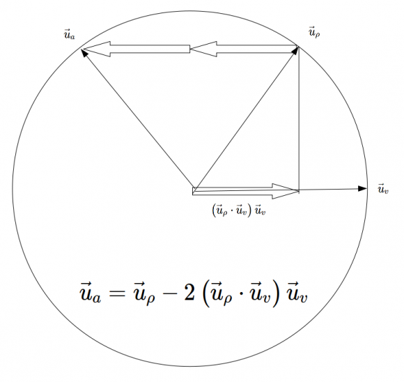
The arrow going to the right shows the direction of the refractive particle as it travels. The arrow slanting upward towards the right points into the thicker $\rho$, or the towards a local source of gravity. The arrow pointing towards the upper left is pointing in the direction of acceleration being felt by the particle.

What is remarkable is that it doesn't matter how fast the particle is going, or how strong the gradient field, the unit directions will always follow this rule. It is also remarkable that the magnitude will always be the same, no matter which direction it goes.

Interpreting it is easy. Imagine the unit gradient of rho vector can swing anywhere around the circle and the velocity unit vector remains fixed. Applying this to a photon flying by the sun. If the photon is heading straight into the sun, the rho vector and the velocity vector will be aligned, so the two leftward hollow arrows would lay on the same axis and point straight backward. This means the photon will be slowing down. If the photon is passing by transversely, the rho vector will point straight upward (or downward) and the acceleration vector will be aligned with it. Once the rho vector swings to the left of the top, the hollow arrows flip and follow the acceleration vector towards the front.

Still crickets from the Academic community.

[ - ]

Comment by Cedron●March 29, 2023

The disparity between (73) and (74) is bigger than it seems. In fact, the G' distinction turns out to be more relevant than the factor of two.

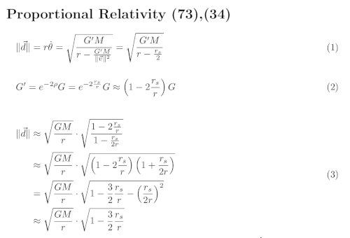
Expanding the G' term changes the nature of the answer from being faster than Newton's ot being slower. GR remains faster.

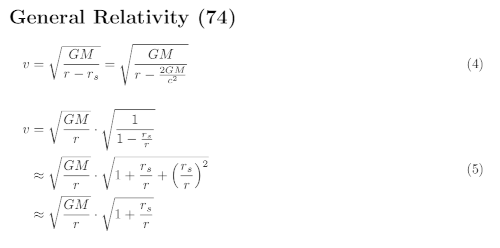
This means if you are observing a system and using Newton's Law to estimate the central mass, you will under estimate the needed mass in the GR case, and over estimate the mass with refractive gravity. Whether the over estimation accounts for all of the need for Dark Matter needs to be resolved.

I consider that Academia's job. If I end up doing it, they will have proven themselves totally worthless.

[ - ]

Comment by Cedron●June 17, 2023

Correction to the Appendix III The Schwarzschild Model. I should have used (19) from [3], not (20). It is even a more complicated equation, however, it gets the zero speed at the Schwarzschild radius instead of a quarter of it, which was a puzzling inconsistency.

Here is the corrected equation with its polynomial approximation for comparison. Calculating $\rho$ and $\vec \nabla \rho$ is ridiculously complicated and not shown.

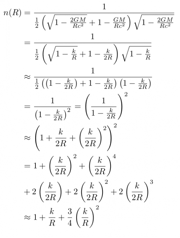
To post reply to a comment, click on the 'reply' button attached to each comment. To post a new comment (not a reply to a comment) check out the 'Write a Comment' tab at the top of the comments.

Please login (on the right) if you already have an account on this platform.

Otherwise, please use this form to register (free) an join one of the largest online community for Electrical/Embedded/DSP/FPGA/ML engineers:

Choose a Username

E-Mail (Work, School or ieee)

First Name

Last Name

Employer

Job Title

Country

State

Password

Confirm Password

By checking this box, I agree with the terms of use and privacy policy By checking this box, I consent to receive occasional emails from the *Related sites and their partners. I understand that these emails will only contain relevant information and that I can unsubscribe at any time.

Off-Topic: A Fluidic Model of the Universe

Introduction

Newtonian Spoken Here

The Speed Equation

Refraction in a Varying Media

Fluff Density

The Refractive Particle Steering Equation

Express with Unit Vectors

The Direction is Magnitude Independent

The Magnitudes are Direction Independent

Permittivity and Permeability

Central Source Point Model

Black Holes Aren't Possible

Convert to a Fluff Scale

Newton's Gravitational Constant

Multiple Sources

Equivalent Single Body

Refraction, not Gravity

Gravitational Force

Motion Enhanced Gravitational Acceleration

The Massive Particle Steering Equation

Sliding Sideways

Comparison to Relativistic Mass

Steering in Polar Coordinates

As Orthogonal Vectors

Free Circular Orbit Velocity

Free Circular Orbit Acceleration

Circular Orbit Radial Limits

Fixed Disk Orbits

Comparison to Simple MOND

Travel Along Gravity Gradient

Nature of the Harness

Toroid Tornadoes

Fluff and Mass

Nature of a Photon

Electrons and Positrons

Electromagnetic Force

Protons and Neutrons

Alpha Particles

Standard Model Generations

Heat

Clocks Slow Down, Time Doesn't

Red Shifts and Blue Shifts

Red Shifts From Far Away

Dark Energy

No Dark Matter

No Big Bang

The Ongoing Creation of Matter

All Sources, No Sinks

In the Long Run

The conjectures employed

Revisiting Einstein's Premises

Conclusion

Appendix I. The Eddington Model

Appendix II. The Dicke Model

Appendix III. Schwarzchild Model

Appendix IV. Comparison to Conjecture

The English Players

The Greek Players

References

Sign in

You might also like...

About Cedron Dawg

Popular Posts by Cedron Dawg

Blogs - Hall of Fame

Free PDF Downloads

Quick Links

About DSPRelated.com

Social Networks

The Related Media Group