


Coupled-Form 2nd-Order IIR Resonators: A Contradiction Resolved
This blog clarifies how to obtain and interpret the z-domain transfer function of the coupled-form 2nd-order IIR resonator. The coupled-form 2nd-order IIR resonator was developed to overcome a shortcoming in the standard 2nd-order IIR resonator. With that thought in mind, let's take a brief look at a standard 2nd-order IIR resonator.
Standard 2nd-Order IIR Resonator
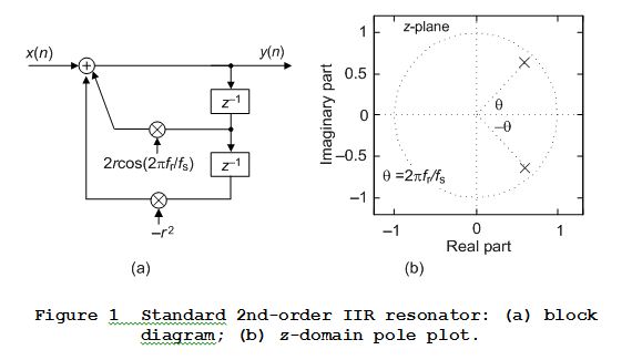
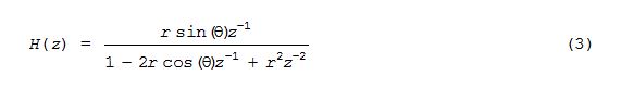
A block diagram of the standard 2nd-order IIR resonator is shown in Figure 1(a). You've probably seen that block diagram many times before. The standard IIR resonator is a type of bandpass resonator with the center of it passband located at fr Hz. (Factor fs is the input data sample rate in Hz.)
The standard IIR resonator's z-domain transfer function is
having two conjugate z-plane poles as shown in Figure 1(b), of radii r, located at angles of ±Θ radians. (The subscript “stand” in Eq. (1) means standard.) Angle Θ is
![]()
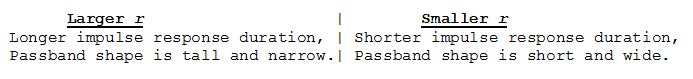
The time-domain impulse response of the standard IIR resonator is a damped sinusoid whose frequency is fr Hz. The amount of damping (the time duration of the damped sinusoid) is determined by the damping factor r, where 0 < r ≤ 1. The damping factor r affects the resonator's impulse response duration, and passband width, as:
The standard IIR resonator has been around for a long time, and is used when someone needs a simple, computationally efficient, bandpass filter. For example, it's used in the implementation of the Goertzel algorithm. OK, you probably know all of this already. Let's move to the main point of this blog.
Quantized Coefficients
With floating point 2rcos(2πfr/fs) and r2 coefficients we can place our resonator's pole wherever we wish on the z-plane. However, in fixed-point processing systems we must quantize those coefficients so as to represent them by binary words having a finite number of binary bits. And in doing so we limit where on the z-plane we can place the resonator's poles. This means we no longer have precise control over the standard resonator's fr resonant frequency or its frequency response shape defined by r.
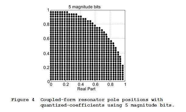
For example, Figure 2(a) shows the mandatory pole positions, in the z-plane's 1st quadrant, when the resonator's coefficients are quantized to 3 magnitude bits. (Due to trigonometric symmetry, the pole locations in the other three quadrants of the z-plane are mirror images of those shown in Figure 2(a).)
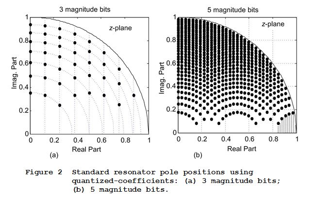
The reason the quantized poles must lie on the intersection of concentric circles and vertical lines is well described in the literature [1-3], so we won't worry about that here.
The key point is that, when using quantized coefficients, we cannot implement the standard Figure 1(a) resonator having relatively low resonant frequencies (poles whose ±Θ angles are near zero radians, i.e., near z = 1). This nonuniform z-plane pole distribution is the reason that low frequency Goertzel filters are difficult to implement. Likewise we cannot implement standard IIR resonators having relatively high resonant frequencies (poles whose ±Θ angles are near π radians, i.e., near z = -1).
This situation improves a little when we quantize our standard resonator's coefficients to a greater number of bits. Figure 2(b) shows the mandatory 1st quadrant pole positions when the coefficients are quantized to 5 magnitude bits. But here again, as shown by the shaded area in Figure 2(b), we are still not able to build a standard resonator that will resonate at a very low (or very high) frequency.
Coupled-Form IIR Resonator
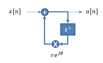
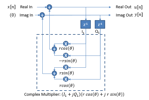
One solution to the above z-plane pole location restrictions is to use what's called the "coupled-form 2nd-order IIR resonator" shown in Figure 3.
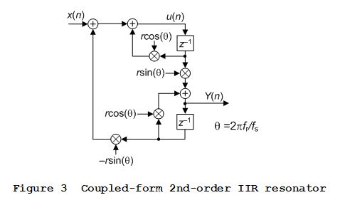
According to two DSP books on my bookshelf [1],[2], the coupled-form IIR resonator has z-plane pole positions, when we quantize the rcos(Θ) and rsin(Θ) coefficients using 5 magnitude bits, as shown in Figure 4. Notice the uniform pole spacing, where poles much closer to z = 1 are now possible. That behavior is what we need to build low-frequency or high-frequency 2nd-order IIR resonators.
Coupled-Form IIR Resonator Transfer Function
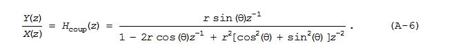
The question I had was, "What is the z-domain transfer function of a coupled-form IIR resonator?" Reference [2] text provided no H(z) expression for the coupled-form resonator, but according to Reference [1] the transfer function of the Figure 3 resonator is:
where, again, Θ = 2rcos(2πfr/fs) radians.
But here's the problem! How can Eq. (3)'s H(z) produce z-plane pole locations that are different from those from Eq. (1)'s Hstand(z) if both expressions have the same denominator polynomial? Something's wrong here.
We resolve this contradiction by realizing, from the derivation provided in the Appendix, that the appropriate transfer function of the coupled-form IIR resonator is:
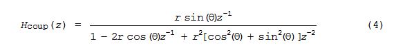
where the subscript "coup" in Eq. (4) means coupled. Next we see that if Eq. (4)'s cos(Θ) and sin(Θ) terms are represented with infinite precision then those terms inside the brackets in the denominator will sum to unity. And in that case the denominator polynomials in Eq. (1), Eq. (3), and Eq. (4) will be identical.
However, when we quantize Figure 3's rcos(Θ) and rsin(Θ)coefficients to some finite number of bits, as we must in our binary world, the r2[cos2(Θ)+sin2(Θ)] factor in the denominator of Eq. (4) will not equal r2. In that case the coefficients of the z-2 terms in the denominators of Eq. (3) and Eq. (4) will be different. And that accounts for the difference in pole locations in Figure 4 compared to Figure 2(b). So the point is, we should always use Eq. (4) to predict the behavior of the coupled-form IIR resonator. This paragraph and Eq. (4) are the most important parts of this blog.
Because I became carried away while writing this blog, and it's longer than it need be, I might as well follow through and present a time-domain example of how the coupled-form IIR resonator is different from the standard IIR resonator.
An IIR Resonator Example
It's straightforward to show how the coupled-form resonator is an improvement over the standard Figure 1(a) resonator. Let's say we want to build a 2nd-order resonator having a resonant frequency of fr = 7 Hz, when our fs sample rate is 400 Hz, and we define our desired damping factor to be r = 0.99. Also we quantize the standard and coupled-form resonators' coefficients (2rcos(2πfr/fs), r2, rcos(2πfr/fs), and rsin(2πfr/fs)) to 5 magnitude bits. The following table shows our quantized-coefficients situation:
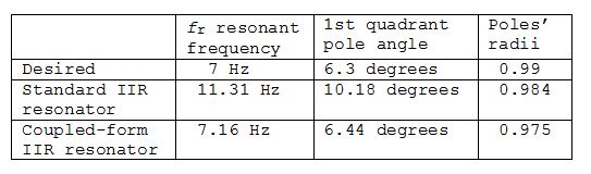
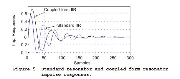
We see from the table that the resonant frequency of the coupled-form resonator is much closer to the desired value of fr = 7 Hz than the resonant frequency of the standard Figure 1(a) resonator. Figure 5 shows the time-domain impulse responses of our two IIR resonators. Notice how the standard resonator oscillates at a much higher frequency than the coupled-form resonator.
OK, the bottom line here is that the coupled-form IIR resonator has better performance than the standard IIR resonator when our desired resonant frequency is very low, or very high, relative to the input data's sample rate. The price we pay for that improved performance is an increase in the number of necessary multiplications per input sample. To quote Forrest Gump, "And that's all I have to say about that."

References
[1] J. Proakis and D. Manolakis, Digital Signal Processing-Principles, Algorithms, and Applications, 3rd Ed., Prentice Hall, Upper Saddle River, New Jersey, 1996, pp. 572–576.
[2] A. Oppenheim and R. Schafer, Discrete-Time Signal Processing, 2nd Ed., Prentice Hall, Englewood Cliffs, New Jersey, 1999, pp. 382–386.
[3] R. Lyons, Understanding Digital Signal Processing, 3rd ed., Prentice Hall, Upper Saddle River, New Jersey, 2011, pp. 833-836.
Appendix
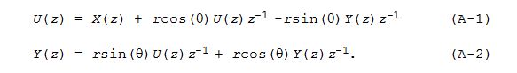
We can obtain the Figure 3 coupled-form resonator's z-domain transfer function by first writing two time-domain equations as:
The z-transforms of those expressions are:
From Eq. (A-1) we can write:
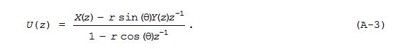
Plugging Eq. (A-3) into Eq. (A-2), we have:
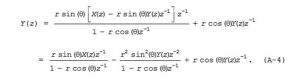
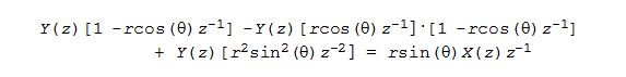
Now we start massaging the heck out of Eq. (A-4) to put Y(z)/X(z) on the left side of an equation and everything else on the right side of that equation. From Eq. (A-4) we write:
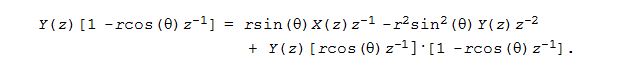
Continuing:
or

and
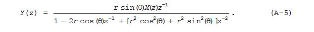
And finally our desired coupled-form Hcoup(z) transfer function is:
- Comments
- Write a Comment Select to add a comment

I just stumbled across this article. I've been using this form for years using a rather shaky combination of intuition and back of the envelope calculations. I hadn't realized that this form was in the literature.
Your article systematizes a lot of what I've been doing by the seat of my pants -- this is cool.

Great write-up Rick! I notice that in your figure 3 if you take y[n] to be right where your u[n] is at the top after the first two adders, you will lose the numerator term such that H_stand(z) and H_coup(z) match (as it is now the difference is a gain and unit sample delay). This made me want to ask if there was any particular reason y[n] is taken instead where it is?

Hi Dan. You’ve asked such a good question!
I chose my Figure 3 coupled resonator’s Y(n) node as the network’s output node merely because that was the output node used by the authors of the books I listed as Reference [1] and [2] of my blog. Since I wrote this blog I’ve learned that Rabiner’s and Gold’s DSP book used my Figure 3’s u(n) node as the output of the network.
{L. Rabiner and B. Gold, "The Theory and Application of Digital Signal Processing", Prentice Hall, Englewood Cliffs, New Jersey, 1975, page 345.}
In their book Rabiner and Gold didn’t give a U(z)/X(x) transfer function for the coupled resonator whose output is the u(n) node. According to my algebra, a coupled resonator whose output is the u(n) node has a z-domain transfer function of:
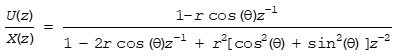 .
.
Dan, two items worth noting with regard to the Figure 3 network:
(I) The Y(n) output in my Figure 3 produces a damped sine impulse response, whereas the u(n) output produces a damped cosine impulse response.
(II) The Figure 3 network works fine as a “resonator” (a simple bandpass filter) when the network’s poles lie inside the z-plane’s unit circle. But that coupled resonator can’t be used as an oscillator (by setting r = 1) because it’s poles cannot (in general) lie exactly on the unit circle.
Thanks Rick for the explanation and your additional points!
You are likely already well aware of this; as a related point of interest I see now as hinted in fred harris' presentation here that the Rader and Gold "Coupled Form" appears to be a single (complex) pole filter with a real input, and we can select the real output, imaginary output, or both as a quadrature signal generation:
Hi Dan.
I've not seen fred harris' paper before. So, no, I was NOT aware of the equivalency of your above two resonator networks. Good job on your part, Dan, in recognizing and pointing that equivalency out to us. How interesting! (Your second network, with its real coefficients, is equivalent to my blog's Figure 3.)
I wonder if the equivalency of your above two resonator networks is the origin (the basis) of Charles Rader's and Ben Gold's "coupled resonator" that they unveiled to the DSP world in their seminal 1967 paper:
Rader and Gold, "Effects of Parameter Quantization on the Poles of a Digital Filter", Proceedings of the IEEE, vol. 55, pp. 688-689, May 1967.
To post reply to a comment, click on the 'reply' button attached to each comment. To post a new comment (not a reply to a comment) check out the 'Write a Comment' tab at the top of the comments.
Please login (on the right) if you already have an account on this platform.
Otherwise, please use this form to register (free) an join one of the largest online community for Electrical/Embedded/DSP/FPGA/ML engineers:


