


Baseband-equivalent phase noise model
Models a noisy local oscillator as found in wireless communications
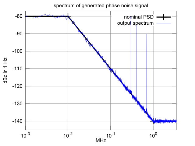
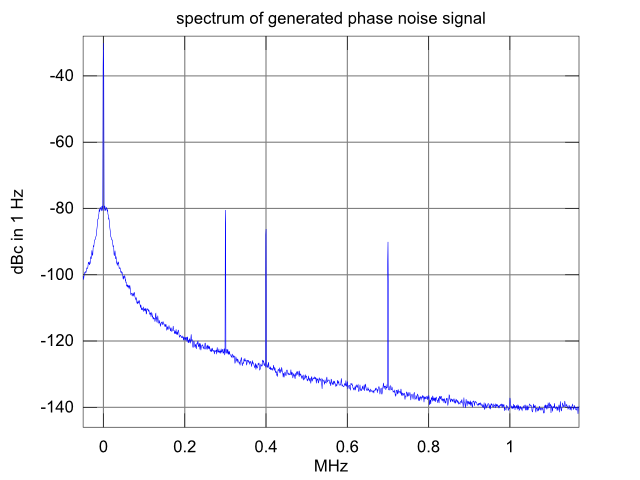
Example output
On a logarithmic frequency axis:
On a linear frequency axis:
Background
In wireless communications, signals are translated to and from radio frequency by multiplication with a local oscillator signal.
Ideally, the local oscillator is a pure sine wave. In reality, it includes a phase noise spectrum that will cause degradation of the wanted signal.
Unfortunately, modeling phase noise is not as straightforward as the usual ”additive white Gaussian noise”:
First, it requires information about the phase noise spectrum, which strongly depends on the application. For example, it is quite different for a base station, a mobile station or a measurement instrument due to different implementation constraints (cost, size, power consumption etc).
Then, given the spectrum, the generation of the phase noise signal as a ”streaming” signal source is not exactly straightforward, because it is difficult to design a reasonably-sized filter that approximates the phase noise spectrum accurately enough.
This code snippet
The code below implements a phase noise source. Based on a phase noise spectrum (and throwing in some discrete spurious tones for added realism), a cyclic phase noise signal is generated and written to file. Full-length FFT filtering avoids the need to design a filter in order to approximate the PN-spectrum.
Cyclic phase noise
The generated phase noise can be used in a simulation or the like. If the data file is too short, it can be wrapped around as many times as needed. A cycle length of a few seconds should be sufficient in typical applications.
Very-low-frequency phase noise is usually not of interest, as it doesn't shift unwanted signals in frequency, and a receiver will remove it from the wanted signal via carrier recovery, frequency-offset correction etc. If necessary, a random-walk process for phase or the like could be added on the simulation side.
Using the phase noise model
Multiply a complex-valued sample stream with the generated phase noise signal.
If the argument includeCarrier is true, the product includes signal and phase noise.
Otherwise (includeCarrier == false), the product will be the isolated phase noise component, for example to visualize the spectrum of the introduced error.
Use with caution, as there may be correlation between PN product and the original signal if the instantaneous phase "wanders" too far from 0 degrees.
Oversampling
Be aware that phase noise products which fall beyond the Nyquist bandwidth will fold back and cause aliasing. Depending on what is being simulated (blockers etc), the simulation may require some ”frequency planning”.
The parameter fMax_Hz will set an upper limit on the generated phase noise (typically ~30 dB reduction, the remaining power beyond fMax_Hz is caused by higher-order sidebands from the nonlinear modulation).
Spurs
The model can generate discrete spurious tones, if desired. Since a continuous-wave signal is infinitely narrow in frequency, the absolute power is specified in dBc (dB relative to carrier) instead of "dBc in 1 Hz" for the phase noise power spectral density.
Finding model parameters
One possibility is to study data sheets and publications on oscillator or synthesizer design. The included example data is by no means intended as "the" phase noise model. As the main purpose is to demonstrate phase noise, it may turn out to be too noisy for some applications.
A division by 2 ideally improves phase noise by 6 dB. For example, a phase noise spectrum published at 1800 MHz could be lowered by 6 dB as a first approximation, if using it at 900 MHz.
As a simple "sanity check", the total phase noise acting on the wanted signal needs to be low enough to reach the maximum SNR required by the radio standard (as a first guess, look up the SNR per symbol here for the modulation in question and an error rate of 1/1000).
Integrated RMS phase error
If needed, this code snippet can be used to calculate the integrated RMS phase error.
Running the code
Copy to "pn_generator.m" and run pn_generator.
The spectrum analyzer (description) can be optionally downloaded here. Copy it into the same directory as pn_generator.m.
% ****************************************************************
% baseband equivalent source of local oscillator with phase noise
% Markus Nentwig, 18.12.2011
% ****************************************************************
function pn_generator()
    close all;

    % ****************************************************************
    % PN generator configuration
    % ****************************************************************
    srcPar = struct();
    srcPar.n = 2 ^ 18; % generated number of output samples
    srcPar.rate_Hz = 7.68e6; % sampling rate
    srcPar.f_Hz = [0, 10e3, 1e6, 9e9]; % phase noise spectrum, frequencies
    srcPar.g_dBc1Hz = [-80, -80, -140, -140]; % phase noise spectrum, magnitude
    srcPar.spursF_Hz = [300e3, 400e3, 700e3]; % discrete spurs (set [] if not needed)
    srcPar.spursG_dBc = [-50, -55, -60]; % discrete spurs, power relative to carrier

    % ****************************************************************
    % run PN generator
    % ****************************************************************
    s = PN_src(srcPar);

    if false
        % ****************************************************************
        % export phase noise baseband-equivalent signal for use in simulator etc
        % ****************************************************************
        tmp = [real(s); imag(s)] .';
        save('phaseNoiseSample.dat', 'tmp', '-ascii');
    end

    if exist('spectrumAnalyzer', 'file')
        % ****************************************************************
        % spectrum analyzer configuration
        % ****************************************************************
        SAparams = struct();
        SAparams.rate_Hz = srcPar.rate_Hz; % sampling rate of the input signal
        SAparams.pRef_W = 1e-3; % unity signal represents 0 dBm (1/1000 W)
        SAparams.pNom_dBm = 0; % show 0 dBm as 0 dB;
        SAparams.filter = 'brickwall';
        SAparams.RBW_window_Hz = 1000; % convolve power spectrum with a 1k filter
        SAparams.RBW_power_Hz = 1; % show power density as dBc in 1 Hz
        SAparams.noisefloor_dB = -250; % don't add artificial noise
        SAparams.logscale = true; % use logarithmic frequency axis

        % plot nominal spectrum
        figure(1); grid on;
        h = semilogx(max(srcPar.f_Hz, 100) / 1e6, srcPar.g_dBc1Hz, 'k+-');
        set(h, 'lineWidth', 3);
        hold on;
        spectrumAnalyzer('signal', s, SAparams, 'fMin_Hz', 100, 'fig', 1);
        ylabel('dBc in 1 Hz');
        legend('nominal PSD', 'output spectrum');
        title('check match with nominal PSD');
        spectrumAnalyzer('signal', s, SAparams, 'fMin_Hz', 100, 'RBW_power_Hz', 'sine', 'fig', 2);
        title('check carrier level (0 dBc); check spurs level(-50/-55/-60 dBc)');
        ylabel('dBc for continuous-wave signal');
        spectrumAnalyzer('signal', s, SAparams, 'fig', 3, 'logscale', false);
        ylabel('dBc in 1 Hz');
    end
end

function pn_td = PN_src(varargin)
    def = {'includeCarrier', true, ...
           'spursF_Hz', [], ...
           'spursG_dBc', [], ...
           'fMax_Hz', []};
    p = vararginToStruct(def, varargin);

    % length of signal in the time domain (after ifft)
    len_s = p.n / p.rate_Hz

    % FFT bin frequency spacing
    deltaF_Hz = 1 / len_s

    % construct AWGN signal in the frequency domain
    % a frequency domain bin value of n gives a time domain power of 1
    % for example ifft([4 0 0 0]) => 1 1 1 1
    % each bin covers a frequency interval of deltaF_Hz
    mag = p.n;

    % scale "unity power in one bin" => "unity power per Hz":
    % multiply with sqrt(deltaF_Hz):
    mag = mag * sqrt(deltaF_Hz);

    % Create noise according to mag in BOTH real- and imaginary value
    mag = mag * sqrt(2);

    % both real- and imaginary part contribute unity power => divide by sqrt(2)
    pn_fd = mag / sqrt(2) * (randn(1, p.n) + 1i * randn(1, p.n));

    % frequency vector corresponding to the FFT bins (0, positive, negative)
    fb_Hz = FFT_freqbase(p.n, deltaF_Hz);

    % interpolate phase noise spectrum on frequency vector
    % note: interpolate dB on logarithmic frequency axis
    H_dB = interp1(log(p.f_Hz+eps), p.g_dBc1Hz, log(abs(fb_Hz)+eps), 'linear');

    % dB => magnitude
    H = 10 .^ (H_dB / 20);
    %    H = 1e-6; % sanity check: enforce flat -120 dBc in 1 Hz

    % apply filter to noise spectrum
    pn_fd = pn_fd .* H;

    % set spurs
    for ix = 1:numel(p.spursF_Hz)
        fs = p.spursF_Hz(ix);
        u = abs(fb_Hz - fs);
        ix2 = find(u == min(u), 1);

        % random phase
        rot = exp(2i*pi*rand());

        % bin value of n: unity (carrier) power (0 dBc)
        % scale with sqrt(2) because imaginary part will be discarded
        % scale with sqrt(2) because the tone appears at both positive and negative frequencies
        smag = 2 * p.n * 10 ^ (p.spursG_dBc(ix) / 20);
        pn_fd(ix2) = smag * rot;
    end

    % limit bandwidth (tool to avoid aliasing in an application
    % using the generated phase noise signal)
    if ~isempty(p.fMax_Hz)
        pn_fd(find(abs(fb_Hz) > p.fMax_Hz)) = 0;
    end

    % convert to time domain
    pn_td = ifft(pn_fd);

    % discard imaginary part
    pn_td = real(pn_td);

    % Now pn_td is a real-valued random signal with a power spectral density
    % as specified in f_Hz / g_dBc1Hz.

    % phase-modulate to carrier
    % note: d/dx exp(x) = 1 near |x| = 1
    % in other words, the phase modulation has unity gain for small phase error
    pn_td = exp(i*pn_td);

    if ~p.includeCarrier
        % remove carrier
        % returns isolated phase noise component
        pn_td = pn_td - 1;
    end
end

% returns a vector of frequencies corresponding to n FFT bins, when the
% frequency spacing between two adjacent bins is deltaF_Hz
function fb_Hz = FFT_freqbase(n, deltaF_Hz)
    fb_Hz = 0:(n - 1);
    fb_Hz = fb_Hz + floor(n / 2);
    fb_Hz = mod(fb_Hz, n);
    fb_Hz = fb_Hz - floor(n / 2);
    fb_Hz = fb_Hz * deltaF_Hz;
end

% *************************************************************
% helper function: Parse varargin argument list
% allows calling myFunc(A, A, A, ...)
% where A is
% - key (string), value (arbitrary) => result.key = value
% - a struct => fields of A are copied to result
% - a cell array => recursive handling using above rules
% *************************************************************
function r = vararginToStruct(varargin)
% note: use of varargin implicitly packs the caller's arguments into a cell array
% that is, calling vararginToStruct('hello') results in
%   varargin = {'hello'}
    r = flattenCellArray(varargin, struct());
end

function r = flattenCellArray(arr, r)
    ix=1;
    ixMax = numel(arr);
    while ix <= ixMax
        e = arr{ix};

        if iscell(e)
            % cell array at 'key' position gets recursively flattened
            % becomes struct
            r = flattenCellArray(e, r);
        elseif ischar(e)
            % string => key.
            % The following entry is a value
            ix = ix + 1;
            v = arr{ix};
            % store key-value pair
            r.(e) = v;
        elseif isstruct(e)
            names = fieldnames(e);
            for ix2 = 1:numel(names)
                k = names{ix2};
                r.(k) = e.(k);
            end
        else
            e
            assert(false)
        end
        ix=ix+1;
    end % while
end


