


The Digital Waveguide Oscillator
In this section, adapted from [460], a digital sinusoidal oscillator derived from digital waveguide theory is described which has good properties for VLSI implementation. Its main features are no wavetable and a computational complexity of only one multiply per sample when amplitude and frequency are constant. Three additions are required per sample. A piecewise exponential amplitude envelope is available for the cost of a second multiplication per sample, which need not be as expensive as the tuning multiply. In the presence of frequency modulation (FM), the amplitude coefficient can be varied to exactly cancel amplitude modulation (AM) caused by changing the frequency of oscillation.
Additive Synthesis
One of the very first computer music techniques introduced was additive synthesis [379]. It is based on Fourier's theorem which states that any sound can be constructed from elementary sinusoids, such as are approximately produced by carefully struck tuning forks. Additive synthesis attempts to apply this theorem to the synthesis of sound by employing large banks of sinusoidal oscillators, each having independent amplitude and frequency controls. Many analysis methods, e.g., the phase vocoder, have been developed to support additive synthesis. A summary is given in [424].
While additive synthesis is very powerful and general, it has been held
back from widespread usage due to its computational expense. For example,
on a single DSP56001 digital signal-processing chip, clocked at 33 MHz,
only about ![]() sinusoidal partials can be synthesized in real time using
non-interpolated, table-lookup oscillators. Interpolated table-lookup
oscillators are much more expensive, and when all the bells and whistles
are added, and system overhead is accounted for, only around
sinusoidal partials can be synthesized in real time using
non-interpolated, table-lookup oscillators. Interpolated table-lookup
oscillators are much more expensive, and when all the bells and whistles
are added, and system overhead is accounted for, only around ![]() fully
general, high-quality partials are sustainable at
fully
general, high-quality partials are sustainable at ![]() KHz on a
KHz on a ![]() DSP56001 (based on analysis of implementations provided by the NeXT Music
Kit).
DSP56001 (based on analysis of implementations provided by the NeXT Music
Kit).
At CD-quality sampling rates, the note A1 on the piano requires
![]() sinusoidal partials, and at least the low-frequency
partials should use interpolated lookups. Assuming a worst-case average of
sinusoidal partials, and at least the low-frequency
partials should use interpolated lookups. Assuming a worst-case average of
![]() partials per voice, providing 32-voice polyphony requires
partials per voice, providing 32-voice polyphony requires ![]() partials, or around
partials, or around ![]() DSP chips, assuming we can pack an average of
DSP chips, assuming we can pack an average of ![]() partials into each DSP. A more reasonable complement of
partials into each DSP. A more reasonable complement of ![]() DSP chips
would provide only
DSP chips
would provide only ![]() -voice polyphony which is simply not enough for a
piano synthesis. However, since DSP chips are getting faster and cheaper,
DSP-based additive synthesis looks viable in the future.
-voice polyphony which is simply not enough for a
piano synthesis. However, since DSP chips are getting faster and cheaper,
DSP-based additive synthesis looks viable in the future.
The cost of additive synthesis can be greatly reduced by making special purpose VLSI optimized for sinusoidal synthesis. In a VLSI environment, major bottlenecks are wavetables and multiplications. Even if a single sinusoidal wavetable is shared, it must be accessed sequentially, inhibiting parallelism. The wavetable can be eliminated entirely if recursive algorithms are used to synthesize sinusoids directly.
Digital Sinusoid Generators
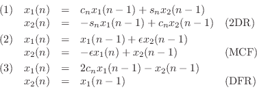
In [168], three techniques were examined for generating sinusoids digitally by means of recursive algorithms.C.12 The recursions can be interpreted as implementations of second-order digital resonators in which the damping is set to zero. The three methods considered were (1) the 2D rotation (2DR), or complex multiply (also called the ``coupled form''), (2) the modified coupled form (MCF), or ``magic circle'' algorithm,C.13which is similar to (1) but with better numerical behavior, and (3) the direct-form, second-order, digital resonator (DFR) with its poles set to the unit circle.
These three recursions may be defined as follows:
The digital waveguide oscillator appears to have the best overall properties yet seen for VLSI implementation. This structure, introduced in [460], may be derived from the theory of digital waveguides (see Appendix C, particularly §C.9, and [433,464]). Any second-order digital filter structure can be used as a starting point for developing a corresponding sinusoidal signal generator, so in this case we begin with the second-order waveguide filter.
The Second-Order Waveguide Filter
The first step is to make a second-order digital filter with zero
damping by abutting two unit-sample sections of waveguide medium, and
terminating on the left and right with perfect reflections, as shown
in Fig.C.38. The wave impedance in section ![]() is given by
is given by
![]() , where
, where ![]() is air density,
is air density, ![]() is the
cross-sectional area of tube section
is the
cross-sectional area of tube section ![]() , and
, and ![]() is sound speed. The
reflection coefficient is determined by the impedance discontinuity
via
is sound speed. The
reflection coefficient is determined by the impedance discontinuity
via
![]() . It turns out that to obtain sinusoidal
oscillation, one of the terminations must provide an inverting
reflection while the other is non-inverting.
. It turns out that to obtain sinusoidal
oscillation, one of the terminations must provide an inverting
reflection while the other is non-inverting.
![\includegraphics[width=\twidth]{eps/wgf}](http://www.dsprelated.com/josimages_new/pasp/img4129.png) |
At the junction between sections ![]() and
and ![]() , the signal is partially
transmitted and partially reflected such that energy is conserved, i.e., we
have lossless scattering. The formula for the reflection
coefficient
, the signal is partially
transmitted and partially reflected such that energy is conserved, i.e., we
have lossless scattering. The formula for the reflection
coefficient ![]() can be derived from the physical constraints that (1)
pressure is continuous across the junction, and (2) there is no net flow
into or out of the junction. For traveling pressure waves
can be derived from the physical constraints that (1)
pressure is continuous across the junction, and (2) there is no net flow
into or out of the junction. For traveling pressure waves ![]() and
volume-velocity waves
and
volume-velocity waves ![]() , we have
, we have
![]() and
and
![]() . The physical pressure and volume velocity are obtained by
summing the traveling-wave components.
. The physical pressure and volume velocity are obtained by
summing the traveling-wave components.
The discrete-time simulation for the physical system of Fig.C.38 is shown in Fig.C.39. The propagation time from the junction to a reflecting termination and back is one sample period. The half sample delay from the junction to the reflecting termination has been commuted with the termination and combined with the half sample delay to the termination. This is a special case of a ``half-rate'' waveguide filter [433].
![\includegraphics[width=\twidth]{eps/dwgf}](http://www.dsprelated.com/josimages_new/pasp/img4134.png)
Since only two samples of delay are present, the digital system is at most
second order, and since the coefficients are real, at most one frequency of
oscillation is possible in ![]() .
.
The scattering junction shown in the figure is called the Kelly-Lochbaum junction in the literature on lattice and ladder digital filters [173]. While it is the most natural from a physical point of view, it requires four multiplies and two additions for its implementation.
It is well known that lossless scattering junctions can be implemented in a
variety of equivalent forms, such as the two-multiply and even one-multiply
junctions. However, most have the disadvantage of not being normalized in the sense that changing the reflection coefficient ![]() changes the amplitude of oscillation. This can be understood physically by
noting that a change in
changes the amplitude of oscillation. This can be understood physically by
noting that a change in ![]() implies a change in
implies a change in ![]() . Since the
signal power contained in a waveguide variable, say
. Since the
signal power contained in a waveguide variable, say ![]() , is
, is
![]() , we find that modulating the reflection coefficient
corresponds to modulating the signal energy represented by the signal
sample in at least one of the two delay elements. Since energy is
proportional to amplitude squared, energy modulation implies amplitude
modulation.
, we find that modulating the reflection coefficient
corresponds to modulating the signal energy represented by the signal
sample in at least one of the two delay elements. Since energy is
proportional to amplitude squared, energy modulation implies amplitude
modulation.
The well-known normalization procedure is to replace the traveling
pressure waves ![]() by ``root-power'' pressure waves
by ``root-power'' pressure waves
![]() so that signal power is just the square of a signal
sample
so that signal power is just the square of a signal
sample
![]() . When this is done, the scattering junction
transforms from the Kelly-Lochbaum or one-multiply form into the
normalized ladder junction in which the reflection coefficients
are again
. When this is done, the scattering junction
transforms from the Kelly-Lochbaum or one-multiply form into the
normalized ladder junction in which the reflection coefficients
are again ![]() , but the forward and reverse transmission
coefficients become
, but the forward and reverse transmission
coefficients become
![]() . Defining
. Defining
![]() , the
transmission coefficients can be seen as
, the
transmission coefficients can be seen as
![]() , and we arrive
essentially at the coupled form, or two-dimensional vector
rotation considered in [168].
, and we arrive
essentially at the coupled form, or two-dimensional vector
rotation considered in [168].
An alternative normalization technique is based on the digital waveguide
transformer (§C.16). The purpose of a ``transformer'' is to
``step'' the force variable (pressure in our example) by some factor ![]() without scattering and without affecting signal energy. Since traveling
signal power is proportional to pressure times velocity
without scattering and without affecting signal energy. Since traveling
signal power is proportional to pressure times velocity ![]() , it
follows that velocity must be stepped by the inverse factor
, it
follows that velocity must be stepped by the inverse factor ![]() to keep
power constant. This is the familiar behavior of transformers for analog
electrical circuits: voltage is stepped up by the ``turns ratio'' and
current is stepped down by the reciprocal factor. Now, since
to keep
power constant. This is the familiar behavior of transformers for analog
electrical circuits: voltage is stepped up by the ``turns ratio'' and
current is stepped down by the reciprocal factor. Now, since
![]() , traveling signal power is equal to
, traveling signal power is equal to
![]() . Therefore,
stepping up pressure through a transformer by the factor
. Therefore,
stepping up pressure through a transformer by the factor ![]() corresponds to
stepping up the wave impedance
corresponds to
stepping up the wave impedance ![]() by the factor
by the factor ![]() . In other words,
the transformer raises pressure and decreases volume velocity by raising
the wave impedance (narrowing the acoustic tube) like a converging cone.
. In other words,
the transformer raises pressure and decreases volume velocity by raising
the wave impedance (narrowing the acoustic tube) like a converging cone.
If a transformer is inserted in a waveguide immediately to the left, say,
of a scattering junction, it can be used to modulate the wave impedance
``seen'' to the left by the junction without having to use root-power waves
in the simulation. As a result, the one-multiply junction can be used for
the scattering junction, since the junction itself is not normalized.
Since the transformer requires two multiplies, a total of three multiplies
can effectively implement a normalized junction, where four were needed
before. Finally, in just this special case, one of the transformer
coefficients can be commuted with the delay element on the left and
combined with the other transformer coefficient. For convenience, the ![]() coefficient on the left is commuted into the junction so it merely toggles
the signs of inputs to existing summers. These transformations lead to the
final form shown in Fig.C.40.
coefficient on the left is commuted into the junction so it merely toggles
the signs of inputs to existing summers. These transformations lead to the
final form shown in Fig.C.40.
![\includegraphics[scale=0.9]{eps/tnwgoAI}](http://www.dsprelated.com/josimages_new/pasp/img4149.png)
The ``tuning coefficient'' is given by
![]() , where
, where
![]() is the desired oscillation frequency in Hz at sample
is the desired oscillation frequency in Hz at sample ![]() (in the
undamped case), and
(in the
undamped case), and ![]() is the sampling period in seconds. The
``amplitude coefficient'' is
is the sampling period in seconds. The
``amplitude coefficient'' is
![]() , where growth or
decay factor per sample (
, where growth or
decay factor per sample (
![]() for constant
amplitude),C.14 and
for constant
amplitude),C.14 and ![]() is the normalizing transformer ``turns
ratio'' given by
is the normalizing transformer ``turns
ratio'' given by
When amplitude and frequency are constant, there is no gradual exponential
growth or decay due to round-off error. This happens because the only
rounding is at the output of the tuning multiply, and all other
computations are exact. Therefore, quantization in the tuning coefficient
can only cause quantization in the frequency of oscillation. Note that any
one-multiply digital oscillator should have this property. In contrast,
the only other known normalized oscillator, the coupled form, does
exhibit exponential amplitude drift because it has two coefficients
![]() and
and
![]() which, after quantization, no longer
obey
which, after quantization, no longer
obey ![]() for most tunings.
for most tunings.
Application to FM Synthesis
The properties of the new oscillator appear well suited for FM
applications in VLSI because of the minimized computational expense.
However, in this application there are issues to be resolved regarding
conversion from modulator output to carrier coefficients. Preliminary
experiments indicate that FM indices less than ![]() are well behaved
when the output of a modulating oscillator simply adds to the
coefficient of the carrier oscillator (bypassing the exact FM
formulas). Approximate amplitude normalizing coefficients have also
been derived which provide a first-order approximation to the exact AM
compensation at low cost. For music synthesis applications, we
believe a distortion in the details of the FM instantaneous frequency
trajectory and a moderate amount of incidental AM can be tolerated
since they produce only second-order timbral effects in many
situations.
are well behaved
when the output of a modulating oscillator simply adds to the
coefficient of the carrier oscillator (bypassing the exact FM
formulas). Approximate amplitude normalizing coefficients have also
been derived which provide a first-order approximation to the exact AM
compensation at low cost. For music synthesis applications, we
believe a distortion in the details of the FM instantaneous frequency
trajectory and a moderate amount of incidental AM can be tolerated
since they produce only second-order timbral effects in many
situations.
Digital Waveguide Resonator
Converting a second-order oscillator into a second-order filter
requires merely introducing damping and defining the input and output
signals. In Fig.C.40, damping is provided by the coefficient
![]() , which we will take to be a constant
, which we will take to be a constant
The foregoing modifications to the digital waveguide oscillator result
in the so-called digital waveguide resonator (DWR)
[304]:
where, as derived in the next section, the coefficients are given by

where
Figure C.41 shows an overlay of initial impulse responses for
the three resonators discussed above. The decay factor was set to
![]() , and the output of each multiplication was quantized to 16
bits, as were all coefficients. The three waveforms sound and look
identical. (There are small differences, however, which can be
seen by plotting the differences of pairs of waveforms.)
, and the output of each multiplication was quantized to 16
bits, as were all coefficients. The three waveforms sound and look
identical. (There are small differences, however, which can be
seen by plotting the differences of pairs of waveforms.)
![\includegraphics[width=\twidth]{eps/tosc16}](http://www.dsprelated.com/josimages_new/pasp/img4188.png) |
Figure C.42 shows the same impulse-response overlay but with
![]() and only 4 significant bits in the coefficients and signals.
The complex multiply oscillator can be seen to decay toward zero due
to coefficient quantization (
and only 4 significant bits in the coefficients and signals.
The complex multiply oscillator can be seen to decay toward zero due
to coefficient quantization (
![]() ). The MCF and DWR remain
steady at their initial amplitude. All three suffer some amount of
tuning perturbation.
). The MCF and DWR remain
steady at their initial amplitude. All three suffer some amount of
tuning perturbation.
![\includegraphics[width=\twidth]{eps/tosc4}](http://www.dsprelated.com/josimages_new/pasp/img4190.png) |
State-Space Analysis
We will now use state-space analysisC.15[449] to determine Equations (C.133-C.136).
![$\displaystyle \left[\begin{array}{c} x_1(n+1) \\ [2pt] x_2(n+1) \end{array}\rig...
...bf{A} \left[\begin{array}{c} x_1(n) \\ [2pt] x_2(n) \end{array}\right] \protect$](http://www.dsprelated.com/josimages_new/pasp/img4193.png)
or, in vector notation,
| (C.137) | |||
| (C.138) |
where we have introduced an input signal
A basic fact from linear algebra is that the determinant of a
matrix is equal to the product of its eigenvalues. As a quick
check, we find that the determinant of ![]() is
is
When the eigenvalues
Note that
![]() . If we diagonalize this system to
obtain
. If we diagonalize this system to
obtain
![]() , where
, where
![]() diag
diag![]() , and
, and
![]() is the matrix of eigenvectors
of
is the matrix of eigenvectors
of
![]() , then we have
, then we have
![$\displaystyle \tilde{\underline{x}}(n) = \tilde{A}^n\,\tilde{\underline{x}}(0) ...
...eft[\begin{array}{c} \tilde{x}_1(0) \\ [2pt] \tilde{x}_2(0) \end{array}\right]
$](http://www.dsprelated.com/josimages_new/pasp/img4209.png)
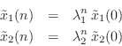
If this system is to generate a real sampled sinusoid at radian frequency
![]() , the eigenvalues
, the eigenvalues ![]() and
and ![]() must be of the form
must be of the form
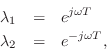
(in either order) where ![]() is real, and
is real, and ![]() denotes the sampling
interval in seconds.
denotes the sampling
interval in seconds.
Thus, we can determine the frequency of oscillation ![]() (and
verify that the system actually oscillates) by determining the
eigenvalues
(and
verify that the system actually oscillates) by determining the
eigenvalues ![]() of
of ![]() . Note that, as a prerequisite, it will
also be necessary to find two linearly independent eigenvectors of
. Note that, as a prerequisite, it will
also be necessary to find two linearly independent eigenvectors of ![]() (columns of
(columns of
![]() ).
).
Eigenstructure
Starting with the defining equation for an eigenvector
![]() and its
corresponding eigenvalue
and its
corresponding eigenvalue ![]() ,
,
![$\displaystyle \left[\begin{array}{cc} gc & c-1 \\ [2pt] gc+g & c \end{array}\ri...
...n{array}{c} {\lambda_i} \\ [2pt] {\lambda_i}\eta_i \end{array}\right]. \protect$](http://www.dsprelated.com/josimages_new/pasp/img4218.png)
We normalized the first element of
Equation (C.141) gives us two equations in two unknowns:
Substituting the first into the second to eliminate
![\begin{eqnarray*}
g+gc+c\eta_i &=& [gc+\eta_i(c-1)]\eta_i = gc\eta_i + \eta_i^2 ...
...{g\left(\frac{1+c}{1-c}\right)
- \frac{c^2(1-g)^2}{4(1-c)^2}}.
\end{eqnarray*}](http://www.dsprelated.com/josimages_new/pasp/img4224.png)
As ![]() approaches
approaches ![]() (no damping), we obtain
(no damping), we obtain
![\begin{eqnarray*}
\underline{e}_1&=&\left[\begin{array}{c} 1 \\ [2pt] \eta \end{...
...t{g\left(\frac{1+c}{1-c}\right)
- \frac{c^2(1-g)^2}{4(1-c)^2}}
\end{eqnarray*}](http://www.dsprelated.com/josimages_new/pasp/img4226.png)
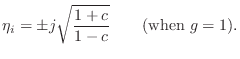
They are linearly independent provided ![]() . In the undamped
case (
. In the undamped
case (![]() ), this holds whenever
), this holds whenever ![]() . The eigenvectors are
finite when
. The eigenvectors are
finite when ![]() . Thus, the nominal range for
. Thus, the nominal range for ![]() is the
interval
is the
interval
![]() .
.
We can now use Eq.![]() (C.142) to find the eigenvalues:
(C.142) to find the eigenvalues:
![\begin{eqnarray*}
{\lambda_i}&=& gc+ \eta_i(c-1)\\
&=& gc+ \frac{(1-g)c}{2}\pm ...
...
\pm j\sqrt{g(1-c^2) - \left[\frac{c(1-g)}{2}\right]^2}
\protect
\end{eqnarray*}](http://www.dsprelated.com/josimages_new/pasp/img4231.png)
Damping and Tuning Parameters
The tuning and damping of the resonator impulse response are governed by the relation
To obtain a specific decay time-constant ![]() , we must have
, we must have
![\begin{eqnarray*}
e^{-2T/\tau} &=& \left\vert{\lambda_i}\right\vert^2 = c^2\left...
...left[g(1-c^2) - c^2\left(\frac{1-g}{2}\right)^2\right]\\
&=& g
\end{eqnarray*}](http://www.dsprelated.com/josimages_new/pasp/img4234.png)
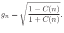
Therefore, given a desired decay time-constant ![]() (and the
sampling interval
(and the
sampling interval ![]() ), we may compute the damping parameter
), we may compute the damping parameter ![]() for
the digital waveguide resonator as
for
the digital waveguide resonator as
To obtain a desired frequency of oscillation, we must solve
![\begin{eqnarray*}
\theta = \omega T
&=& \tan^{-1}\left[\frac{\sqrt{g(1-c^2) - [...
...,\tan^2{\theta} &=& \frac{g(1-c^2) - [c(1-g)/2]^2}{[c(1+g)/2]^2}
\end{eqnarray*}](http://www.dsprelated.com/josimages_new/pasp/img4236.png)
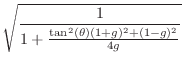
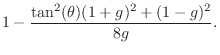
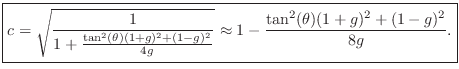
for ![]() , which yields
, which yields
Eigenvalues in the Undamped Case
When ![]() , the eigenvalues reduce to
, the eigenvalues reduce to
where
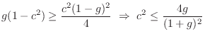
For
![]() , the eigenvalues are real, corresponding to
exponential growth and/or decay. (The values
, the eigenvalues are real, corresponding to
exponential growth and/or decay. (The values ![]() were
excluded above in deriving Eq.
were
excluded above in deriving Eq.![]() (C.144).)
(C.144).)
In summary, the coefficient ![]() in the digital waveguide oscillator
(
in the digital waveguide oscillator
(![]() ) and the frequency of sinusoidal oscillation
) and the frequency of sinusoidal oscillation ![]() is simply
is simply
Summary
This section introduced and analyzed the digital waveguide oscillator and resonator, as well as some related algorithms. As a recursive algorithm for digital sinusoid generation, it has excellent properties for VLSI implementation. It is like the 2D rotation (complex multiply) in that it offers instantaneous amplitude from its state and constant amplitude in the presence of frequency modulation. However, its implementation requires only two multiplies per sample instead of four. When used as a constant-frequency oscillator, it requires only one multiply per sample.
Matlab Sinusoidal Oscillator Implementations
This section provides Matlab/Octave program listings for the sinusoidal resonator/oscillator algorithms discussed above:
- Planar 2D Rotation (2DR) (``complex multiply'')
- Modified Coupled Form (MCF) (``Magic Circle'')
- Digital Waveguide Resonator (DWR)
% Filter test program in matlab

%N = 300;   % Number of samples to generate
N = 3000;   % Number of samples to generate
f = 100;   % Desired oscillation frequency (Hz)
fs = 8192; % Audio sampling rate (Hz)
%R = .99;   % Decay factor (1=never, 0=instant)
R = 1;   % Decay factor (1=never, 0=instant)
b1 = 1;    % Input gain to state variable x(n)
b2 = 0;    % Input gain to state variable y(n)

%nd = 16;   % Number of significant digits to use
nd = 4;   % Number of significant digits to use
base = 2;  % Mantissa base (two significant figures)
           % (see 'help chop' in Matlab)

u = [1,zeros(1,N-1)]; % driving input test signal
theta = 2*pi*f/fs; % resonance frequency, rad/sample

% ================================================
% 2D PLANAR ROTATION (COMPLEX MULTIPLY)

x1 = zeros(1,N); % Predeclare saved-state arrays
y1 = zeros(1,N);

x1(1) = 0;      % Initial condition
y1(1) = 0;      % Initial condition

c = chop(R*cos(theta),nd,base); % coefficient 1
s = chop(R*sin(theta),nd,base); % coefficient 2

for n=1:N-1,
  x1(n+1) = chop(   c*x1(n) - s*y1(n) + b1*u(n), nd,base);
  y1(n+1) = chop(   s*x1(n) + c*y1(n) + b2*u(n), nd,base);
end

% ================================================
% MODIFIED COUPLED FORM ("MAGIC CIRCLE")
% (ref: http://ccrma.stanford.edu/~jos/wgo/ )

x2 = zeros(1,N); % Predeclare saved-state arrays
y2 = zeros(1,N);

x2(1) = 0.0;     % Initial condition
y2(1) = 0.0;     % Initial condition

e = chop(2*sin(theta/2),nd,base); % tuning coefficient

for n=1:N-1,
  x2(n+1) = chop(R*(x2(n)-e*y2(n))+b1*u(n),nd,base);
  y2(n+1) = chop(R*(e*x2(n+1)+y2(n))+b2*u(n),nd,base);
end

% ================================================
% DIGITAL WAVEGUIDE RESONATOR (DWR)

x3 = zeros(1,N); % Predeclare saved-state arrays
y3 = zeros(1,N);

x3(1) = 0;      % Initial condition
y3(1) = 0;      % Initial condition

g = R*R;        % decay coefficient
t = tan(theta); % toward tuning coefficient
cp = sqrt(g/(g + t^2*(1+g)^2/4 + (1-g)^2/4)); % exact
%cp = 1 - (t^2*(1+g)^2 + (1-g)^2)/(8*g); % good approx
b1n = b1*sqrt((1-cp)/(1+cp)); % input scaling

% Quantize coefficients:
cp = chop(cp,nd,base);
g = chop(g,nd,base);
b1n = chop(b1n,nd,base);

for n=1:N-1,
  gx3 = chop(g*x3(n), nd,base); % mpy 1
  y3n = y3(n);
  temp = chop(cp*(gx3 + y3n), nd,base); % mpy 2
  x3(n+1) = temp - y3n + b1n*u(n);
  y3(n+1) = gx3 + temp + b2*u(n);
end

% ================================================
% playandplot.m

figure(4);
title('Impulse Response Overlay');
ylabel('Amplitude');
xlabel('Time (samples)');
alt=1;%alt = (-1).^(0:N-1); % for visibility
plot([y1',y2',(alt.*y3)']); grid('on');
legend('2DR','MCF','WGR');
title('Impulse Response Overlay');
ylabel('Amplitude');
xlabel('Time (samples)');

saveplot(sprintf('eps/tosc%d.ps',nd));

if 1
  playandplot(y1,u,fs,'2D rotation',1);
  playandplot(y2,u,fs,'Magic circle',2);
  playandplot(y3,u,fs,'WGR',3);
end

function playandplot(y,u,fs,ttl,fnum);
% sound(y,fs,16);
  figure(fnum);

  unwind_protect # protect graph state
  subplot(211);
  axis("labely");
  axis("autoy");
  xlabel("");
  title(ttl);
  ylabel('Amplitude');
  xlabel('Time (ms)');
  t = 1000*(0:length(u)-1)/fs;
  timeplot(t,u,'-');
  legend('input');
  subplot(212);
  ylabel('Amplitude');
  xlabel('Time (ms)');
  timeplot(t,y,'-');
  legend('output');
  unwind_protect_cleanup # restore graph state
    grid("off");
    axis("auto","label");
    oneplot();
  end_unwind_protect
endfunction
Note that the chop utility only exists in Matlab. In Octave, the following ``compatibility stub'' can be used:
function [y] = chop(x,nd,base)
y = x;
Faust Implementation
The function oscw (file osc.lib) implements a digital waveguide sinusoidal oscillator in the Faust language [453,154,170]. There is also oscr implementing the 2D rotation case, and oscs implementing the modified coupled form (magic circle).
Next Section:
Non-Cylindrical Acoustic Tubes
Previous Section:
Waveguide Transformers and Gyrators


