Sign in

Search Online Books

Free Online Books

Sponsor

Industry's highest performing at the lowest power DSPs now as low as $5.00*
Start development today!
*volume pricing for 10ku

Chapters

Physical Audio Signal Processing
    Digital Waveguide Theory
       The Dispersive 1D Wave Equation
          Higher Order Terms

Chapter Contents:

Search Physical Audio Signal Processing

Book Index | Global Index

Would you like to be notified by email when Julius Orion Smith III publishes a new entry into his blog?

Higher Order Terms

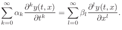
The complete, linear, time-invariant generalization of the lossy, stiff string is described by the differential equation

$\displaystyle \sum_{k=0}^\infty \alpha_k \frac{\partial^k y(t,x)}{\partial t^k} = \sum_{l=0}^\infty \beta_l \frac{\partial^l y(t,x)}{\partial x^l}. \protect$

(C.33)

which, on setting $y(t,x) = e^{st+vx}$ , (or taking the 2D Laplace transform with zero initial conditions), yields the algebraic equation,

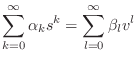$\displaystyle \sum_{k=0}^\infty \alpha_k s^k = \sum_{l=0}^\infty \beta_l v^l$

(C.34)

Solving for

in terms of

is, of course, nontrivial in general. However, in specific cases, we can determine the appropriate attenuation per sample $G(\omega)$ and wave propagation speed $c(\omega)$ by numerical means. For example, starting at

, we normally also have

(corresponding to the absence of static deformation in the medium). Stepping

forward by a small differential $j{{\Delta}}\omega$ , the left-hand side can be approximated by $\alpha_0+\alpha_1j{{\Delta}}\omega$ . Requiring the generalized wave velocity

to be continuous, a physically reasonable assumption, the right-hand side can be approximated by $\beta_0+\beta_1 \Delta v$ , and the solution is easy. As

steps forward, higher order terms become important one by one on both sides of the equation. Each new term in

spawns a new solution for

in terms of

, since the order of the polynomial in

is incremented. It appears possible that homotopy continuation methods [316] can be used to keep track of the branching solutions of

as a function of

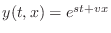
. For each solution

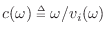
, let ${v_r}(\omega)$ denote the real part of $v(j\omega)$ and let ${v_i}(\omega)$ denote the imaginary part. Then the eigensolution family can be seen in the form $\exp{\left\{j\omega t\pm v(j\omega)x\right\}}=\exp{\left\{\pm{v_r}(\omega)x\right\}}\cdot\exp{\left\{j\omega\left(t \pm {v_i}(\omega)x/\omega\right)\right\}}$ . Defining $c(\omega)\isdeftext \omega/{v_i}(\omega)$ , and sampling according to $x\to x_m\isdeftext mX$ and $t\to t_n\isdeftext nT(\omega)$ , with $X\isdeftext c(\omega)T(\omega)$ as before, (the spatial sampling period is taken to be frequency invariant, while the temporal sampling interval is modulated versus frequency using allpass filters), the left- and right-going sampled eigensolutions become

$\displaystyle e^{j\omega t_n\pm v(j\omega)x_m}$	$\displaystyle =$	$\displaystyle e^{\pm{v_r}(\omega)x_m}\cdot e^{ j\omega\left(t_n\pm x_m/c(\omega)\right)}$	(C.35)
	$\displaystyle =$	$\displaystyle G^m(\omega)\cdot e^{ j\omega\left(n \pm m\right)T(\omega)}$

where $G(\omega)\isdef e^{\pm{v_r}(\omega)X}$ . Thus, a general map of

versus

, corresponding to a partial differential equation of any order in the form (C.33), can be translated, in principle, into an accurate, local, linear, time-invariant, discrete-time simulation. The boundary conditions and initial state determine the initial mixture of the various solution branches as usual.

We see that a large class of wave equations with constant coefficients, of any order, admits a decaying, dispersive, traveling-wave type solution. Even-order time derivatives give rise to frequency-dependent dispersion and odd-order time derivatives correspond to frequency-dependent losses. The corresponding digital simulation of an arbitrarily long (undriven and unobserved) section of medium can be simplified via commutativity to at most two pure delays and at most two linear, time-invariant filters.

Every linear, time-invariant filter can be expressed as a zero-phase filter in series with an allpass filter. The zero-phase part can be interpreted as implementing a frequency-dependent gain (damping in a digital waveguide), and the allpass part can be seen as frequency-dependent delay (dispersion in a digital waveguide).

Previous: The Dispersive 1D Wave Equation
Next: Alternative Wave Variables

Order a Hardcopy of Physical Audio Signal Processing

About the Author: Julius Orion Smith III
Julius Smith's background is in electrical engineering (BS Rice 1975, PhD Stanford 1983). He is presently Professor of Music and Associate Professor (by courtesy) of Electrical Engineering at Stanford's Center for Computer Research in Music and Acoustics (CCRMA), teaching courses and pursuing research related to signal processing applied to music and audio systems. See http://ccrma.stanford.edu/~jos/ for details.

Comments

No comments yet for this page

Add a Comment

You need to login before you can post a comment (best way to prevent spam). ( Not a member? )