


Loaded Waveguide Junctions
In this section, scattering relations will be derived for the general
case of N waveguides meeting at a load. When a load is
present, the scattering is no longer lossless, unless the load itself
is lossless. (i.e., its impedance has a zero real part). For ![]() ,
,
![]() will denote a velocity wave traveling into the junction,
and will be called an ``incoming'' velocity wave as opposed to
``right-going.''C.9
will denote a velocity wave traveling into the junction,
and will be called an ``incoming'' velocity wave as opposed to
``right-going.''C.9
![\includegraphics[width=\twidth]{eps/fNstrings}](http://www.dsprelated.com/josimages_new/pasp/img3925.png) |
Consider first the series junction of ![]() waveguides
containing transverse force and velocity waves. At a series junction,
there is a common velocity while the forces sum. For definiteness, we
may think of
waveguides
containing transverse force and velocity waves. At a series junction,
there is a common velocity while the forces sum. For definiteness, we
may think of ![]() ideal strings intersecting at a single point, and the
intersection point can be attached to a lumped load impedance
ideal strings intersecting at a single point, and the
intersection point can be attached to a lumped load impedance
![]() , as depicted in Fig.C.29 for
, as depicted in Fig.C.29 for ![]() . The presence of
the lumped load means we need to look at the wave variables in the
frequency domain, i.e.,
. The presence of
the lumped load means we need to look at the wave variables in the
frequency domain, i.e.,
![]() for velocity waves and
for velocity waves and
![]() for force waves, where
for force waves, where
![]() denotes
the Laplace transform. In the discrete-time case, we use the
denotes
the Laplace transform. In the discrete-time case, we use the ![]() transform instead, but otherwise the story is identical. The physical
constraints at the junction are
transform instead, but otherwise the story is identical. The physical
constraints at the junction are
| (C.90) | |||
| (C.91) |
where the reference direction for the load force
The parallel junction is characterized by
| (C.92) | |||
| (C.93) |
For example,
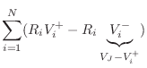
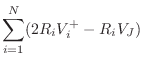
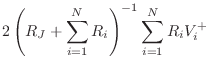
The scattering relations for the series junction are derived as
follows, dropping the common argument `![]() ' for simplicity:
' for simplicity:
 |
(C.94) | ||
 |
(C.95) | ||
 |
(C.96) |
where
(written to be valid also in the multivariable case involving square impedance matrices
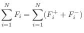
Finally, from the basic relation
Similarly, the scattering relations for the loaded parallel junction
are given by
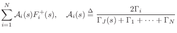
where
It is interesting to note that the junction load is equivalent to an
![]() st waveguide having a (generalized) wave impedance given by the
load impedance. This makes sense when one recalls that a transmission
line can be ``perfectly terminated'' (i.e., suppressing all
reflections from the termination) using a lumped resistor equal in
value to the wave impedance of the transmission line. Thus, as far as
a traveling wave is concerned, there is no difference between a wave
impedance and a lumped impedance of the same value.
st waveguide having a (generalized) wave impedance given by the
load impedance. This makes sense when one recalls that a transmission
line can be ``perfectly terminated'' (i.e., suppressing all
reflections from the termination) using a lumped resistor equal in
value to the wave impedance of the transmission line. Thus, as far as
a traveling wave is concerned, there is no difference between a wave
impedance and a lumped impedance of the same value.
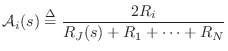
In the unloaded case, ![]() , and we can return to the time
domain and define (for the series junction)
, and we can return to the time
domain and define (for the series junction)
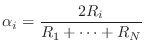
These we call the alpha parameters, and they are analogous to those used to characterize ``adaptors'' in wave digital filters (§F.2.2). For unloaded junctions, the alpha parameters obey
| (C.103) |
and
 |
(C.104) |
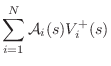
In the unloaded case, the series junction scattering relations are given (in
the time domain) by

The alpha parameters provide an interesting and useful parametrization of waveguide junctions. They are explicitly the coefficients of the incoming traveling waves needed to compute junction velocity for a series junction (or junction force or pressure at a parallel junction), and losslessness is assured provided only that the alpha parameters be nonnegative and sum to
Note that in the lossless, equal-impedance case, in which all waveguide
impedances have the same value ![]() , (C.102) reduces to
, (C.102) reduces to
When, furthermore,
An elaborated discussion of ![]() strings intersection at a load is
given in in §9.2.1. Further discussion of the digital waveguide
mesh appears in §C.14.
strings intersection at a load is
given in in §9.2.1. Further discussion of the digital waveguide
mesh appears in §C.14.
Next Section:
Two Coupled Strings
Previous Section:
Properties of Passive Impedances


